How do demosceners create complex computer animations in just a few kilobytes? One of our secret weapons is Shader Minifier, a tool that minifies GLSL code. Over the years, it has evolved to pack more data into tiny executables, pushing the boundaries of what’s possible. In this blog post, we’ll go through its evolution.
In 2010, I noticed a trend in the demoscene: creators were producing impressive 4k intros, but the process was incredibly manual and tedious. These intros relied on shader code to generate graphics, and optimizing this code was like a code golf competition. As the existing tooling was poor, I decided to help. My goal was to automate the most boring tasks: removing unnecessary spaces and comments, and renaming variables to a single letter. This is how Shader Minifier was born.
The compression paradox
One of the first features I implemented was the insertion of preprocessor macros. This is a classic trick often used in code golf competitions and obfuscation contests:
#define R return
By adding this line at the top of your code, you can replace every instance of “return” with “R”, saving 5 bytes per statement. This can quickly add up, especially if you apply it to other common keywords or standard function calls.
But someone once asked me: “Shader Minifier makes files small, but how many bytes does it actually save after compression with Crinkler?” Crinkler is the most popular compression tool for small intros.
At first, I didn’t care much: if I make the code smaller, the compressed code will obviously get smaller too… right? Nope, I was wrong. I tested it and I found out that the output of Shader Minifier was compressing to something bigger than the non-minified code. Was it bad luck? I experimented and adjusted some heuristics in the code. Is it best to introduce more macros or fewer? After multiple iterations, I found that the best approach was… to do nothing. Do not replace code with macros.
Turns out, Crinkler is smarter than I thought, and my clever macros were getting in its way. Modern compressors are excellent at identifying redundant patterns. If the word “return” is repeated throughout the code, the compressor can handle it very efficiently. Using macros to eliminate these redundancies is counterproductive.
Renaming: not as easy as ABC
Renaming identifiers seems like an obvious feature for a minifier. Initially, the goal seemed simple: use a single letter for each identifier. After all, one letter per identifier is optimal, right? Yet again, I was mistaken. Not all letters are equal when it comes to compression.
A good name is one that you reuse. If multiple variables have the same name, the code will look more repetitive and compress better.
So our strategy is to be pretty aggressive in reusing names:
Variables in two different functions can obviously use the same name.
If a global variable is not referenced within a function, we can also reuse its name thanks to variable shadowing.
We can even reuse function names. With function overloading, the compiler will distinguish them as long as they have different arguments.
Yep. We’ve been so aggressive in reusing names that we’ve discovered bugs in glslang:
When a minifier breaks your compiler, you know you’re pushing boundaries.
Reducing the number of unique variable names is very effective. But you also have to pick good names. Should we name the variable “V” or “A”? Experiments show that picking one name or the other can affect the compressed size. It’s hard to know which name will perform better, but we compute the frequencies of letters and bigrams to guess which names are more likely to be better. The idea is to look at which characters appear more often in the rest of the code, and which pairs of characters are already common. In the end, it’s just a heuristic, and we could probably do better.
With these features implemented, my original goal was achieved. Many demosceners have been using Shader Minifier for years to create their mind-blowing 4k intros.
But one day, I decided to create my first 8k intro. The story behind The Sheep and the Flower was detailed in the blog post “How we made an animated movie in 8kB”.
Size-coding and code golfing are fun when there’s a small amount of code. But as the codebase grows beyond 1,000 lines, micro-optimizations become increasingly painful. The problem is that we also need to maintain and iterate on the code, so it needs to remain readable throughout the development of the intro. To be able to sheep my intro, more features were needed in Shader Minifier.
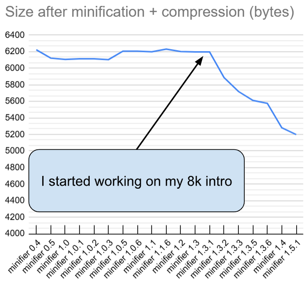
Here’s a graph showing the evolution:
This graph shows the evolution of Shader Minifier and how big my 47kB shader code will get after minification plus compression. Without minification, Crinkler compresses the code down to about 10kB. I compared around 20 different versions of Shader Minifier and compressed their output with Crinkler to track the tool’s evolution.
So the recent improvements to Shader Minifier have saved about 1kB on this specific shader (between version 1.3 and 1.5). But don’t focus too much on this number: some of the improvements are about quality-of-life, not raw size. For example, it’s nice that we no longer have to manually find and remove unused functions.
In case you wonder about the size regression in version 1.0.5: at that time, we lacked proper tests for compression, so it went unnoticed (it was something related to renaming heuristics). Testing infrastructure is something that we improved later. Anyway, the point is that 47kB became 5.2kB after minifier and compression magic. The rest of the 8kB are filled with the music and the setup code.
So, what have we done since version 1.3?
Static analysis
We used static analysis and implemented features commonly found in optimizing compilers.
The full list of optimizations is long, it includes many micro-optimizations and things like GLSL vectors and swizzles transformations. If you’re curious, check the documentation for a more detailed list of optimizations.
Below are some of the most impactful optimizations. You’ll notice how they try to reduce the number of names we need. Whether it’s variables or functions, each time we can get rid of an identifier, we help make the code more compressible.
Inlining
If a variable is used only once, we can inline it and eliminate the declaration.
Even if used multiple times, trivial constants like 0.5 or vec3(1) are often better inlined.
Variables reuse
In some cases, we reuse a variable name instead of declaring a new one, assuming they don’t overlap.
For example, this code:
vec3 x = vec3(.2);
# use x
# …
vec3 col=vec3(0,.04,.04);
Can be converted to:
vec3 x = vec3(.2);
// use x
// …
x=vec3(0,.04,.04);
Functions
Shader Minifier can inline small functions and remove arguments that always receive the same value.
For example, Shader Minifier will detect that the corner argument is not really needed here:
What started as a simple tool 15 years ago has grown into something more sophisticated. In recent years, our goal has been to simplify the development of 8k intros and make the process more enjoyable. With Shader Minifier, you can achieve much more without spending countless hours on micro-optimizations.
I hope the graph above will encourage users to upgrade their version of Shader Minifier. Quite often, people will download it once and keep it for years. New versions can help you squeeze more into your executable. This is especially true when you have non-trivial amounts of code.
But it’s not over. How well does Shader Minifier perform when creating a 64k intro? These larger intros come with their own set of challenges, often involving multiple shaders that we have to minify together. While Shader Minifier can already save multiple kilobytes, there are still many opportunities for improvement…
We’ll look into this. There are bytes still waiting to be saved.
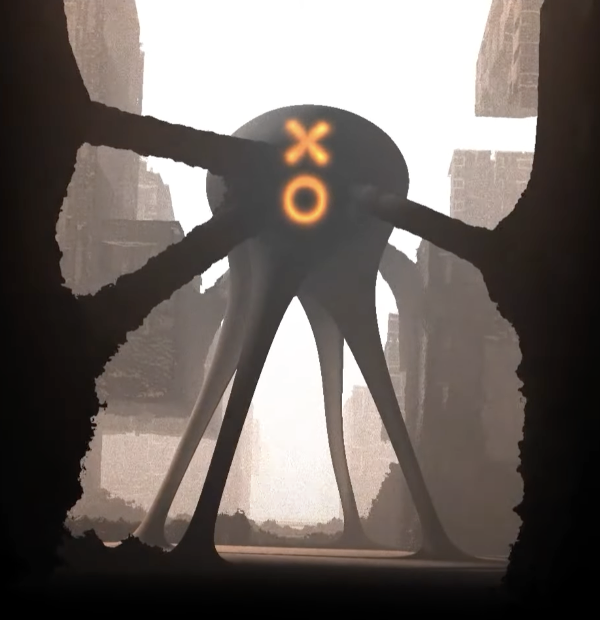
In November 2022, we set ourselves a challenge: make a real-time animation that looks like a standard short animated movie, with the constraint that it should fit in 8 kilobytes. The goal was to have decent graphics, animations, direction and camera work, and the matching music… Yes, 8 kilobytes, less than half of this post, for everything. It wasn’t clear how much was actually feasible, so we had to try it.
In April 2023, after months of work, we finally released The Sheep and the Flower. You can run it by yourself (download link), or see a YouTube capture of the program running:
Many people asked how we were able to create something like this. This article will explain the technical details and design constraints behind this production. We’ve also made the source code public on GitHub.
Overview
The result is a Windows executable file. It’s a single .exe file that generates everything. It requires no resource file, no external depency, except for Windows and up-to-date drivers.
Here’s the quick summary of what we used. We’ll explain the details in the rest of the post.
All the visuals are computed in real-time on the GPU, using GLSL shaders. This includes the timeline information, camera setup, etc.
The rendering is done with raymarching.
The shaders are minified using my own tool, Shader Minifier.
The music was composed using OpenMPT and the 4klang synthesizer, which generates an assembly file able to replay the music. The instruments are described procedurally, while the list of notes is simply compressed.
The code was written in C++ using Visual Studio 2022.
To get started with the compiler flags and initialization, we used the Leviathan framework.
One day, I saw a message from a former colleague, who shared a video he made a long time ago, called Capoda. I immediately loved the concept. The content is simple, yet it manages to tell a story efficiently.
I shared the link with some friends and thought it could be a good example of a story suitable for size coding. I was about to add this concept to the list of cool things I’ll probably never do, when Anatole replied:
Looks like a perfect fit for 8kb ! Will you do it? I have always dreamed of making a prod like this, but I’m waiting for the “good and original idea”.
I was excited by the project because I wanted to do more demos with story-telling and animations. At the same time, I was intrigued by the challenges of making something in 8kB: I usually target 64kB, which is a completely different world, with a different set of rules and challenges. For the music, I knew I could count on my old friend CyborgJeff. Anatole had a lot of experience with 4kB. With him, the project was much more likely to be successful. And that’s how we started working together. I was not certain it would be feasible to fit everything in 8kB, but there’s only one way to know, right?
Why specifically 8kB? In the demoscene, there are multiple size categories, with 4kB and 64kB being very common. I’ve always enjoyed the techniques used in 4kB intros (an intro is a demo with a tight size limitation), but it always feels too limited for proper storytelling. Revision, the biggest demoparty in the world, added an 8kB competition a few years ago, so it was a good opportunity to try it.
Rendering Worlds with Two Triangles
People familiar with the demoscene already know it, as this is a standard approach since 2008: we draw a rectangle (so, two triangles) to cover the full screen. Then, we run a GPU program (called a shader) on the rectangle using the GLSL language. The program will compute a color for each pixel and each frame. All we need is a function that takes coordinates (and time) as input, and returns a color. Simple, right?
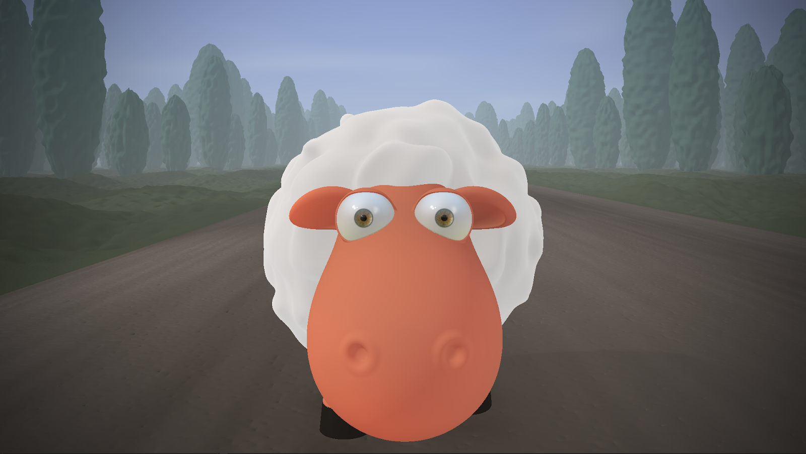
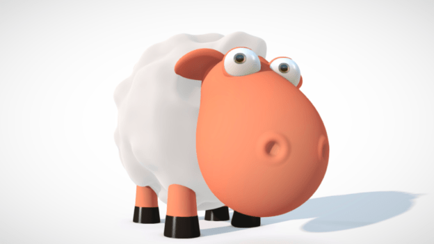
“Please draw me a sheep!” — Antoine de Saint-Exupéry, The Little Prince
Of course, the big question is: how do we write a function that draws a sheep?
Let’s split the problem in two parts:
Represent the scene as a signed distance field.
Use raymarching to convert the distance fields into pixels.
Signed Distance Fields (SDF)
A distance field is a function that computes the distance between a point in space to the nearest object. For every point in space, we want to know how far the point is to the object. If a point is one the object’s surface, the function should return 0. This is a “signed” function, meaning that it will return a negative number for points inside the object.
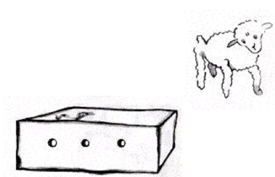
In the most basic cases, the function is simple to write. For example, the distance between a point and a sphere is trivial to compute. For a cube, you can also do it in a couple of lines (see The SDF of a Box for explanations). Lots of other building blocks have been documented. Inigo Quilez has a nice collection of simple reusable shapes and the Mercury demo group also provides a great library.
The true power of distance fields emerges when you combine them. To get the union of two objects, you can simply pick the minimum of the two distances, while the maximum gives the intersection. When crafting organic shapes, mathematical unions may appear coarse, but alternative formulas like the smooth unions can create more organic looks.
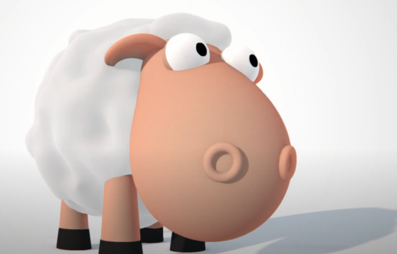
Once you have a toolset with building blocks, it feels like playing with legos to create an object or a scene. Thus we made our sheep by assembling simple shapes (for example a cone, a sphere) and merging them, while the body and wool consist of a 3D noise function.
The next task will be to actually render the distance function to the screen.
Raymarching
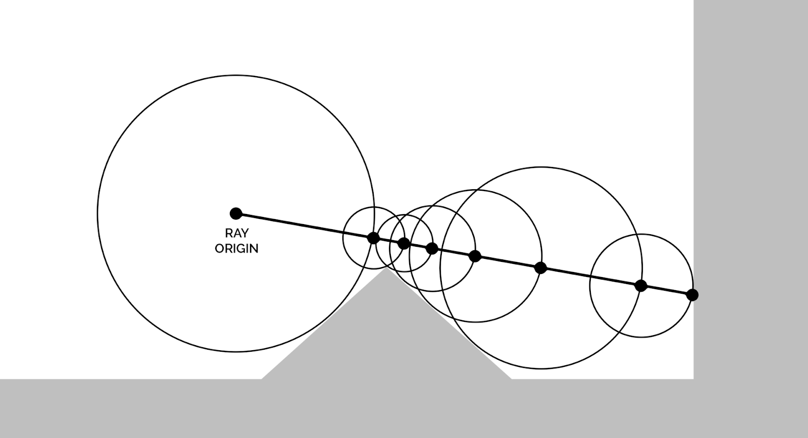
To draw the 3D scene on the screen, we use raymarching. Raymarching is a rendering technique that leverages SDFs to trace rays through a 3D scene. Unlike traditional ray tracing, which mathematically computes the intersection point, raymarching works by marching along the ray’s path. The SDF tells us how far we can walk without colliding with the scene. We can then move the ray origin and compute the new distance. We repeat the operation until the distance is 0 (or close to it).
In the image below, imagine that the ray origin is the camera. It is looking in a certain direction. After multiple iterations, we find the intersection point with the right wall.
Once we have the intersection point, we know if the current pixel should be a part of the sheep, the sky, or any other object. For the lighting, we need to know at least the surface normal, which we can estimate by computing the gradient in the same area. To compute shadows, we can send another ray for the point to the sun and find if an object is in between. Many techniques exist to improve the rendering quality beyond this basic idea.
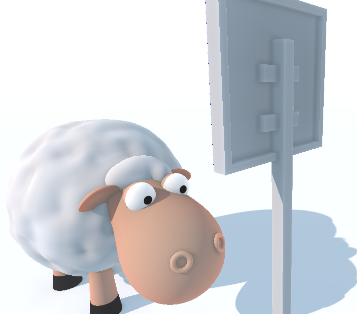
Imagine that you have to tell a story, but there is only one character, with no voice or written text, and that character is barely animated. It can only walk (but not turn!), move the head and the eyes. With only this, how would you tell a story and convey emotions?
When creating a demo with such a small size limit, it’s critical to know what is important. We avoided anything that didn’t serve that story. For example, we originally imagined the sheep walking in a desert. It wouldn’t be hard to generate dunes and a sky, but the story didn’t actually need it. We decided to keep the pure white background. We also skipped the textures, except for a few that convey a meaning (like the signs and the eyes).
Keeping the scope of the work relatively small allowed us to focus on things that might not be obvious at first: the details and the polish, the camera work, the editing, and the synchronization. Each shot was manually crafted, each animation was adjusted and went through many iterations to make sure the flow feels right. Not only did we need to make sure the flow felt right (adjusting the length of the shots and the sequencing), but it had to match the music.
To ensure that the narrative resonates with the audience, we employed a number of storytelling techniques, often with redundancy for emphasis. For example, to show the sheep’s excitement, we used cartoonish 2D effects, accelerated the walking pace, accentuated tail movements, exaggerated head swings, and added a dramatic shift in the music. This approach allowed us to convey a spectrum of emotions throughout the story.
The camera itself is also a storytelling tool. We used a wide shot to evoke a sense of solitude when the sheep wanders for hours; an extreme closeup on its eyes to capture the moment of realization when it notices the sign; and a slow zoom on the head to intensify the focus when the sheep stares at a sign.
A 2D animated background was used to communicate the appeal of the flower.
Development process
You may notice that the source code contains a large number of hard-coded constants. The challenge was to determine these values — how large should the sheep’s eyes be? How fast should the camera move? How long should each shot last? What colors should the flower have?
Given this uncertainty, each constant went through numerous iterations. To iterate quickly and have a short feedback loop, shaders come in handy: we recompile them at runtime to update the graphics within a second.
The other requirement was to have a player: something that allows us to control the time with pause and replay commands. This proved to be invaluable when working on animations and camera control, as we could see the result instantly after a live-reload of the shader. Additionally, music support was a must, so that we can perfectly synchronize the animations to the music. We designed our early prototypes in Shadertoy, but we later transitioned to KodeLife, and finally moved the code to our own project (in C++, using a small framework called Leviathan).
Music
Music is a critical component for storytelling. To fit the story, the music needed multiple parts, with different moods and transitions at specific points in time. We decided to use the same tools as we would in a 4kB intro, while allocating more space to allow a more intricate composition.
To compose the music, I asked my Cyborgjeff, a friend familiar with demoscene techniques, whose musical style resonated with our vision. His tool of choice was the 4klang synthesizer, an impressive piece of software developed by Gopher. 4klang comes with a plugin usable from any music software and it has an export button that generates an assembly file. This file is then compiled and linked with the demo. When the demo runs, the synth will run in a separate thread, procedurally generate the wave sound, and send it to the soundcard.
Creating a small music comes with a lot of constraints. The first version of the music was bigger than expected. Imagine telling a musician “Your music is too big, can you reduce it by 500 bytes?” Well, that’s just normal in the demoscene.
We studied the output of 4klang to understand how it packs the data. With advice from Gopher, Cyborgjeff was able to iterate on the music to make it smaller. We made multiple adjustments:
The number of instruments was reduced from 16 to 13.
The ending theme was recomposed to align with the tempo of the overall music.
The composition used more repetitions so it compresses better. For example, adjusting the length of a note in the background may be imperceptible to the ear while improving the compression ratio.
This allowed us to save some space on the music, while keeping its overall structure, with a minimal loss in terms of quality. For more information on the music, Cyborgjeff wrote a blog post: 8000 octets, un mouton et une fleur.
Animation & Synchronization
Everything in the demo is re-evaluated at each frame as nothing is precomputed or cached. While this is really bad for the performance, this is a blessing for animations: anything can depend on the time and vary through the demo.
The demo consists of around 25 manually crafted camera shots. When creating a shot, we describe how each of 18 parameters varies over time, such as the position of each object, the state of the sheep, the position of the camera, the focal, what the camera is looking at, etc.
For example, a single line of code describes the camera during the shot:
camPos = vec3(22., 2., time*0.6-10.);
And we get a linear translation. Here “time” represents the time since the beginning of the shot so that we can easily insert, remove or adjust a shot without affecting the rest of the demo. Absolute times are avoided for code maintenance.
A note of caution on linear interpolations: while functional, they often look poor or robotic. In many cases, we apply the smoothstep function, which leads to a smoother, more natural animation. Smoothstep is an S-shaped smooth interpolation that helps avoid sharp edges and sudden movement changes. The code for the timeline is in the vertex shader. You may notice that each shot is defined in a similar way, and the code may seem redundant. It’s not a problem, as redundancy leads to better compression.
Textures & Materials
In a traditional renderer, textures are 2D images that are applied on a 3D model. One difficulty with the textures is how to compute the texture coordinates and map each pixel in the texture to the 3D surface. With our raymarching approach, we can’t easily compute texture coordinates. Instead, we compute on the fly 3D textures. Once the raymarcher finds the 3D position of the point to render, we pass the 3D coordinates to the corresponding texture function.
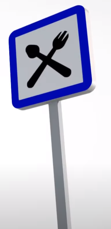
Let’s take a look at the traffic signs. They use some math to compute a triangle or a square to serve as a border, then the inner content of the sign is achieved by combining multiple functions. For example, the restaurant symbol is created with 4 black oval-like shapes, and 2 white shapes are added to create the dents.
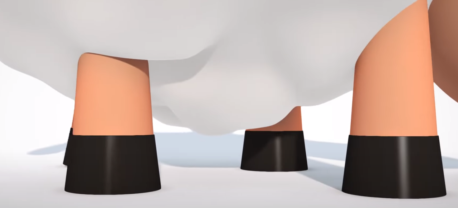
To make the visuals more interesting, we wanted to have not just textures, but also different materials. Parameters of the lighting equation depend on the material. For example, the sheep hooves have a different reflection (using fresnel coefficients).
Eyes
For a long time during the development, the eyes looked dull and lifeless. I believe eyes are a big part of the character design. This was one of the first things that we animated, and it was very important as a tool for story-telling. Eyes help show feelings and they enable many transitions.
Early rendering
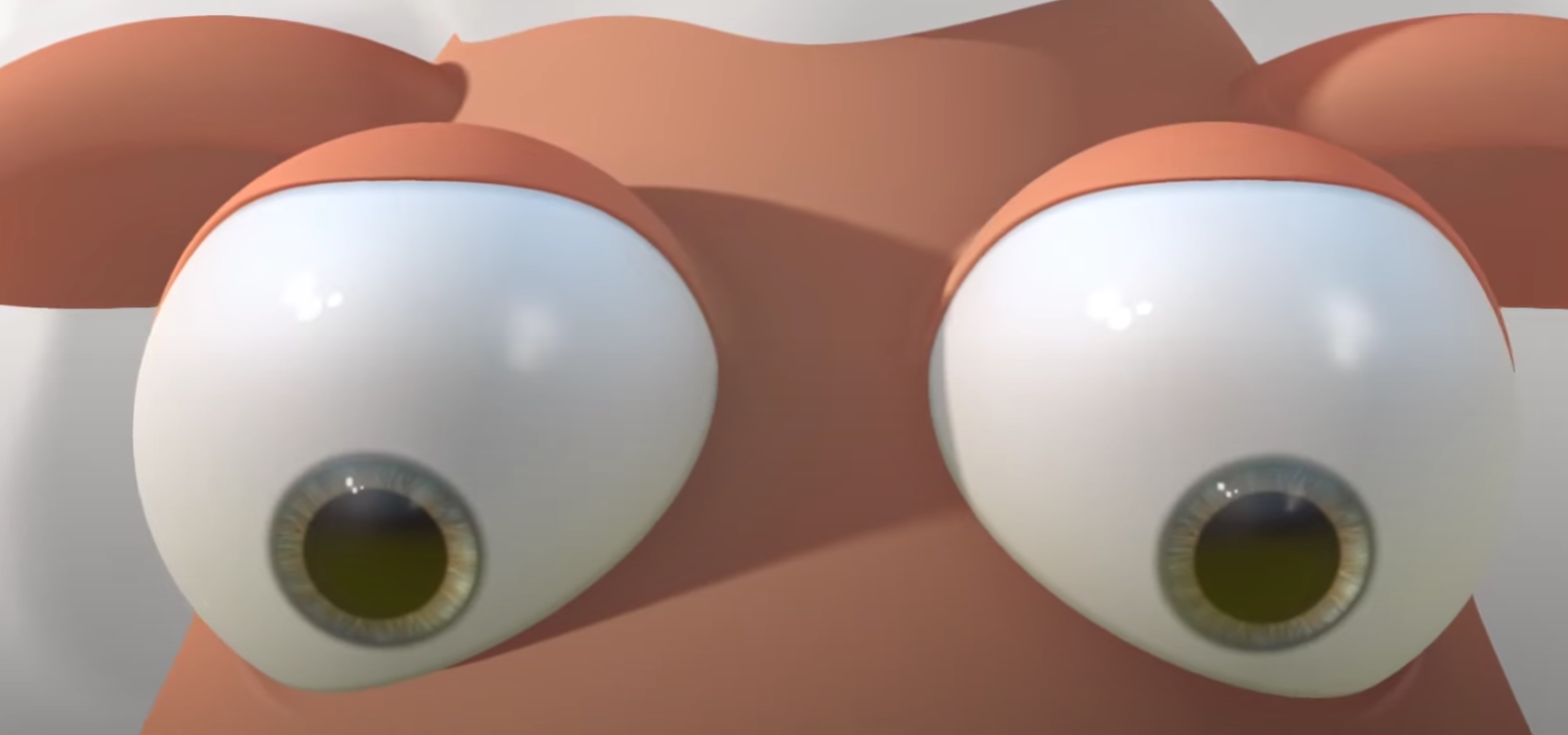
After searching for reference images on the Internet, I found that most of the cartoon characters have an iris, but the iris doesn’t seem to be strictly required. I’ve also noticed that the pupil is always big. If there’s an iris, the pupil will be big compared to the iris.
But the important part to get sparkling eyes is to have some reflections of the light in the eyes. With the standard lighting equations we used, we couldn’t get a reflection (unless the sun and the camera were at very specific positions). An input of the lighting equations is the normal vector of the surface. Our trick was to modify the vector to increase the probability of getting some reflections from the sun.
On top of that, we created an environment mapping. This technique is commonly used in video games: instead of computing perfect reflections in the scene in real time, we can look up in a texture (that simulates the environment). Usually, people use environment mapping to optimize the code as the texture can be a simplification of the real environment. We did the opposite: our environment world is actually a perfect white, but we used a texture to fake and add details.
Final result
The reflections in the eyes (both the white and the pupils) are much more complex than they should be in an empty world. There are multiple fake sources of lights, as well as a gradient (to mimic a darker ground and a blue-ish sky).
Post-processing
Once everything is done, the final visual touch defining the mood is the post-processing.
Despite being subtle, it helps have a good image quality and set the tone for the story. We used:
color grading;
gamma correction;
a bit of vignetting;
finally, a two-pass FXAA filter to avoid aliasing (but you won’t notice it if you only watched the YouTube capture)
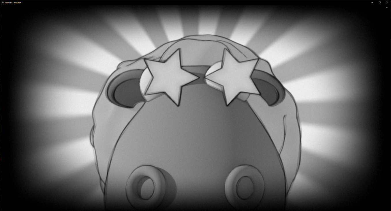
We also implemented some of the effects in the post-processing step, such as the stars in the eyes or the ending screen effect. Those are made as pure 2D and don’t exist in the 3D world.
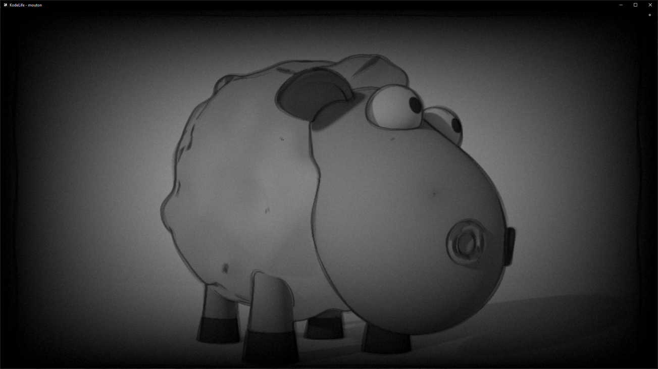
Finally, we experimented with other alternative styles. At some point, we tried to give an old-cartoon look, and we implemented contour detection to simulate a hand-drawn image, with a monochrome rendering, grain, and noise. The result looked like this:
After discussions, we decided to give up on this experiment and focus on the cleaner, modern look.
Compression
So far, we’ve seen how we made most of the demo. The main idea is to avoid storing data, instead we use code to describe how to generate the data. For the music, we store a list of notes to play, as well as a list of instructions for each instrument. All of this is relatively small, but does it really fit in 8kB?
Part of the magic comes from Crinkler, a compression tool specifically designed for the demoscene and intros between 1kB and 8kB. As the executable needs to be self-extractible, Crinkler includes some very small and clever assembly code that can decompress the rest of the executable. It’s optimized for size at the expense of other things: the compression algorithm takes a while, the decompression is relatively slow and uses a lot of RAM (hundreds of megabytes).
Crinkler is an impressive tool, but it doesn’t do everything. We have a total of 42kB of shader source code and we need one last ingredient to fit it in the binary.
Minification
As the shader source code is included in the final binary, we have to make it as small as possible. It would be possible to minify the code by hand, but then it would cause maintenance issues. It was critical for the success of our project to be able to iterate quickly, without worrying about low-level size optimizations. So we needed a tool to minify the shader.
I have written such a tool, Shader Minifier, which has been a side project of mine since 2011. It removes unneeded spaces and comments, it renames variables and can do more. It has been the most popular shader minification tool in the demoscene for many years, but this was not sufficient for us: an 8kB intro contains much more code than a 4kB does, and new problems arise from the larger code size.
I stopped working on the demo for one month to implement all the missing features we needed from Shader Minifier. While it’s easy to write a simple minifier, you need to write a compiler if you want to get good minification — a source-to-source compiler, similar to what Closure Compiler does.
The full list of transformations supported by Shader Minifier is getting quite long, but here are a few:
Renaming of variables and functions
Inlining of variables
Evaluation of constant arithmetic
Inlining of functions
Dead code elimination
Merging of declarations
These transformations reduce the size of the output, but it’s not enough. We need to make sure that the output is compression-friendly. This is a hard problem: it can happen that a transformation reduces the size of the code, while increasing the size of the compressed code. So we constantly need to monitor the compressed size, as we iterate on the demo.
New improvements to Shader Minifier have saved around 600 bytes on the compressed binary. To help review and monitor what exactly goes in the final binary, we store the minified output in the repository. This proved useful to identify new optimization opportunities. At the end, once minified and compressed, the 42kB of shader code fits in about 5kB, which gives just enough space for the music and the C++ code.
Anyway… you could say that I had to write a compiler in order to make this demo. :)
The War Between the Sheep and the Flowers
It’s not important, the war between the sheep and the flowers? […] Suppose I happen to know a unique flower, one that exists nowhere in the world except on my planet, one that a little sheep can wipe out in a single bite one morning, just like that, without even realizing what he’d doing – that isn’t important? If someone loves a flower of which just one example exists among all the millions and millions of stars, that’s enough to make him happy when he looks at the stars. He tells himself ‘My flower’s up there somewhere…’ But if the sheep eats the flower, then for him it’s as if, suddenly, all the stars went out. And that isn’t important?”
— Antoine de Saint-Exupéry, The Little Prince
Conclusion
As you’ve seen, there are lots of advanced and fascinating techniques needed to make this kind of demo. But we didn’t invent everything. We’re building on top of what other people did. The amount of work and research that was done by other people is incredible, from the raymarching techniques, to the music generation software and the compression algorithms. Hopefully the new features added to Shader Minifier will help other people create better demos in the future. The 8kB category is fun and offers more possibilities than the 4kB category; let’s hope it will become more popular.
P.S. For comparison, the text of this article contains around 21,000 characters, so it would take 21kB.
In the previous part, we saw how textures are generated in H – Immersion. This time, we’ll have a look at another important tool for size coding: procedural geometry.
More specifically, since our rendering uses traditional polygons, we wrote a procedural mesh generator. We’ll see how with a few well chosen techniques, it is possible to create a variety of shapes, or make a viewer believe we did.
First, Cubes
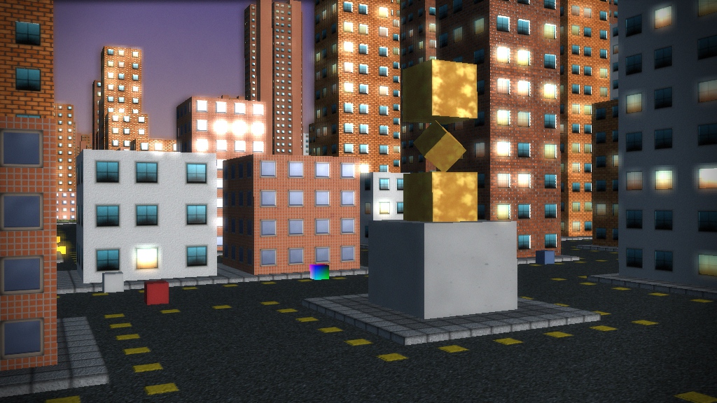
When we started making demos, the 64kB limit felt intimidating. We didn’t know anything about procedural mesh generation, and we already had a lot to do with the rendering, the camera, the textures, the story… well, with everything. So in our first demo, B – Incubation, we took the early decision to skip 3D modeling altogether. Instead, we chose to use only cubes and designed the demo around this concept.
This is an example of how a technical constraint can become a creative challenge, and force us to look for new ideas and do something unexpected. In all of our 64kB intros, the size limitation affects the design, sometimes in small and unexpected ways: we are constantly looking for tricks, code reuse, and workarounds to evade this barrier.
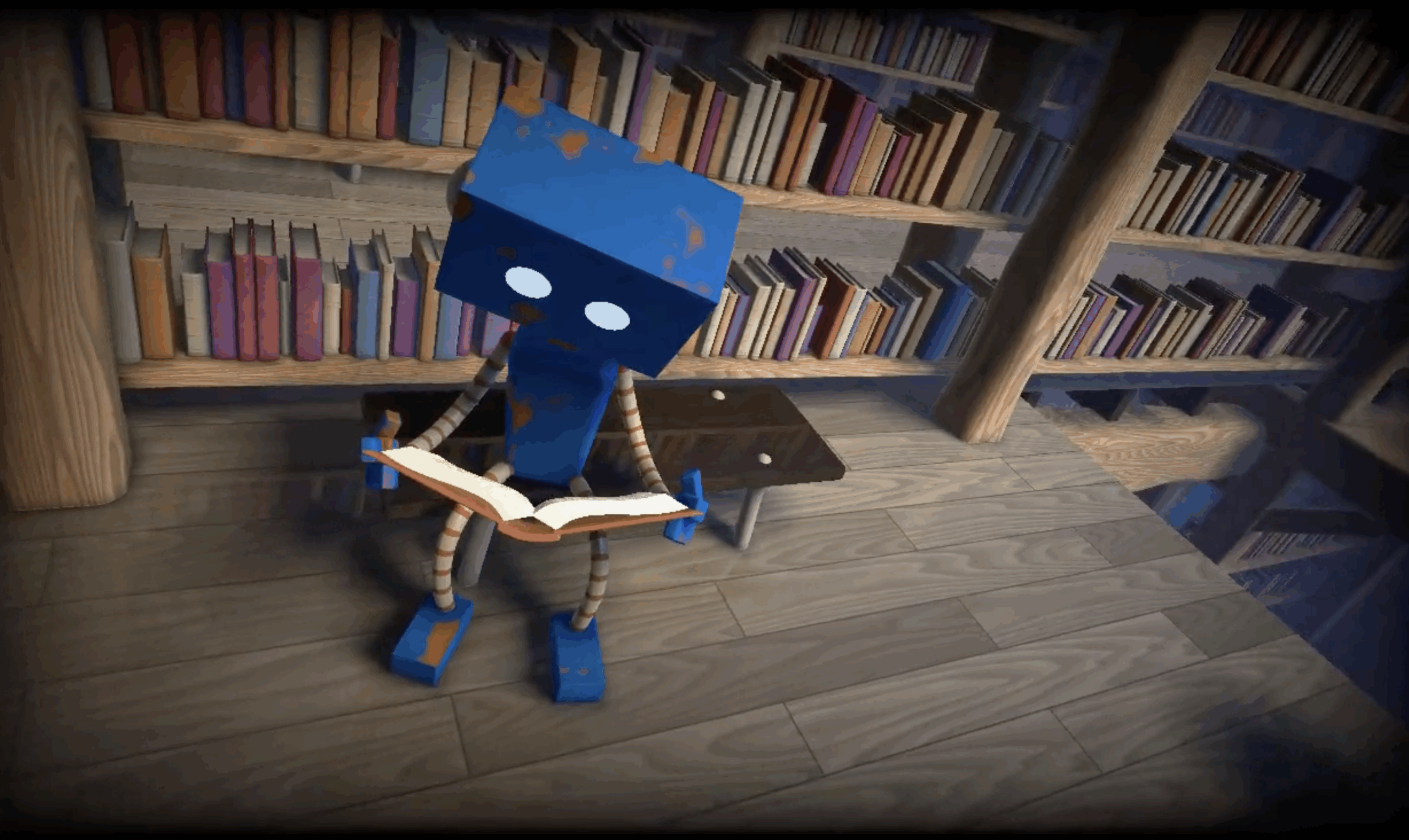
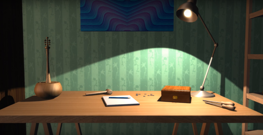
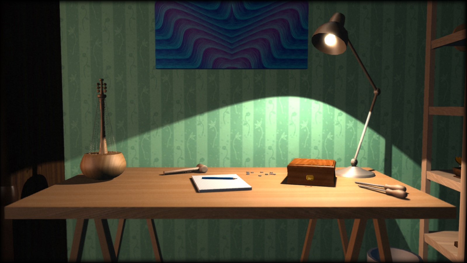
After this first 64kB, it was time to introduce procedural meshes at last! For F – Felix’s Workshop, we implemented some rudimentary mesh generation. The demo received good feedback, but the code is probably simpler than what many people expect.
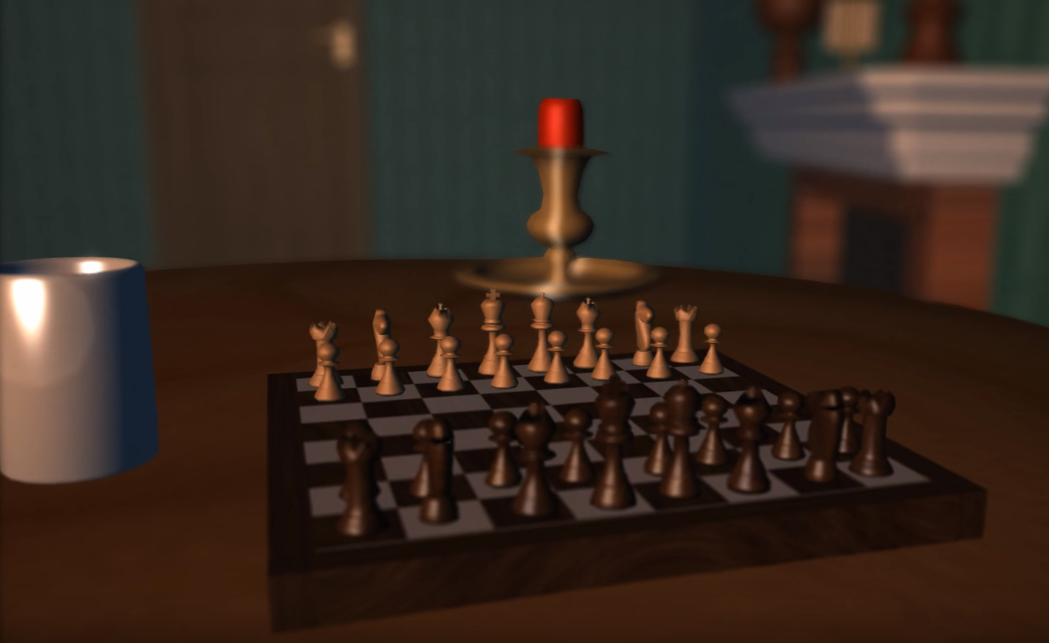
If you pay close attention to the image below, you might notice that there are only two kinds of shapes used by all geometry. Some elements, like the table, the shelf and the wall, are made by assembling deformed cubes. The rest have varied shapes, but are all sort of cylindrical. Indeed we built them using surfaces of revolution.
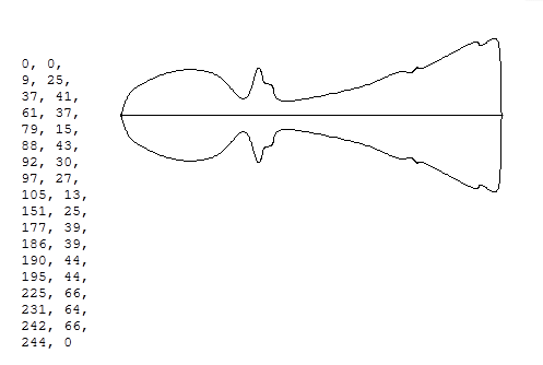
The idea is to draw simple splines, then rotate them around an axis to create 3D models. Here is the spline we used to create pawns on a chessboard.
The numbers on the left are 2D coordinates of a list of control points. We interpolate between the points using Catmull-Rom splines. Catmull-Rom is a nice algorithm first published in 1974, which Iñigo Quilez details and recommends. The shape on the right is the result (after symmetry) of applying the technique on the list of points.
Once done, we can convert the data to 3D by creating faces along the spline. With little variation we can also create other chess pieces. Here’s the final result.
How many bytes do we need for this? Not too many, especially when you reuse the technique in lots of ways throughout the demo. If we stored each number on one byte, we would need less than 40 bytes of data to represent the pawn… and this doesn’t take into account the compression step.
If you look at the source code for the chessboard, you’ll notice that we actually use a floating-point type to store these integers between 0 and 255. These 32-bit floats use 4 bytes each. Is it a waste of bytes? Not quite: as said in the previous paragraph, the program is compressed. If you check the binary representation of those floats, you’ll see they are very similar and end with a bunch of 0s. The compression tool (kkrunchy) will pack this efficiently, and it can be smaller than if we tried to be smart. Going further, delta encoding could improve compression rates, but it only becomes beneficial when there’s enough data to store. There’s more to say about floats, and we’ve touched the topic before in the article Making floating point numbers smaller.
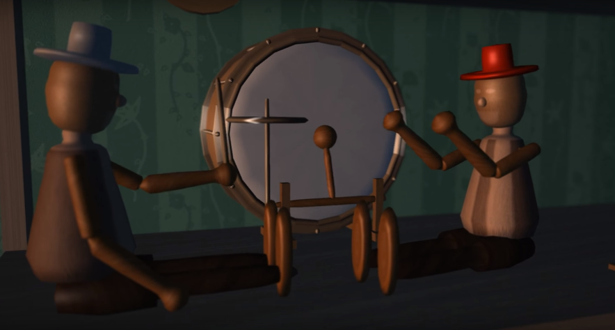
In the scene above, notice how the drum has distinct faces. Our function lets us control the number of faces to generate, so not everything has to be perfectly circular. For example, the pencil on the desk is hexagonal.
In the background of the chess scene, even the white ornament at the top of the hearth is made with this technique: it is built as a pointy octogonal shape. Then the central part is elongated along one axis, resulting in a large shape with beveled corners. We can not only elongate the shape along an axis, but also generate it along a curve. This is how the train ramp is made, with its path described by another spline. If you watch again Felix’s Workshop, you can see how everything comes either from a revolution or from a cube. We create a wide range of objects just by combining these two primitives.
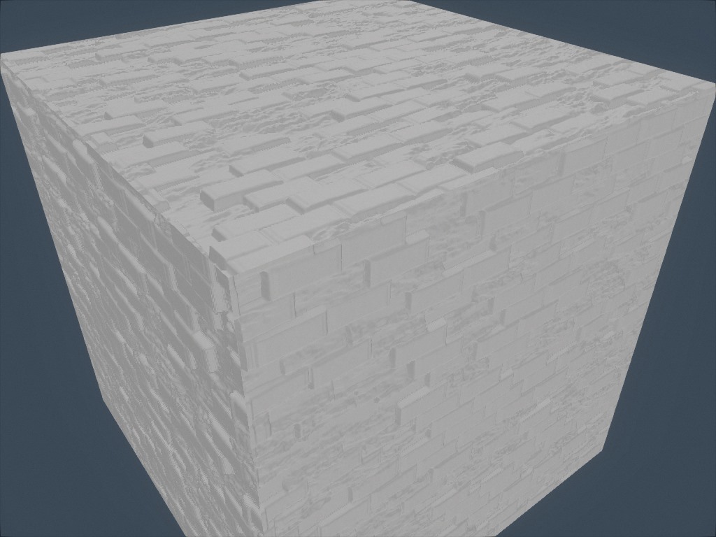
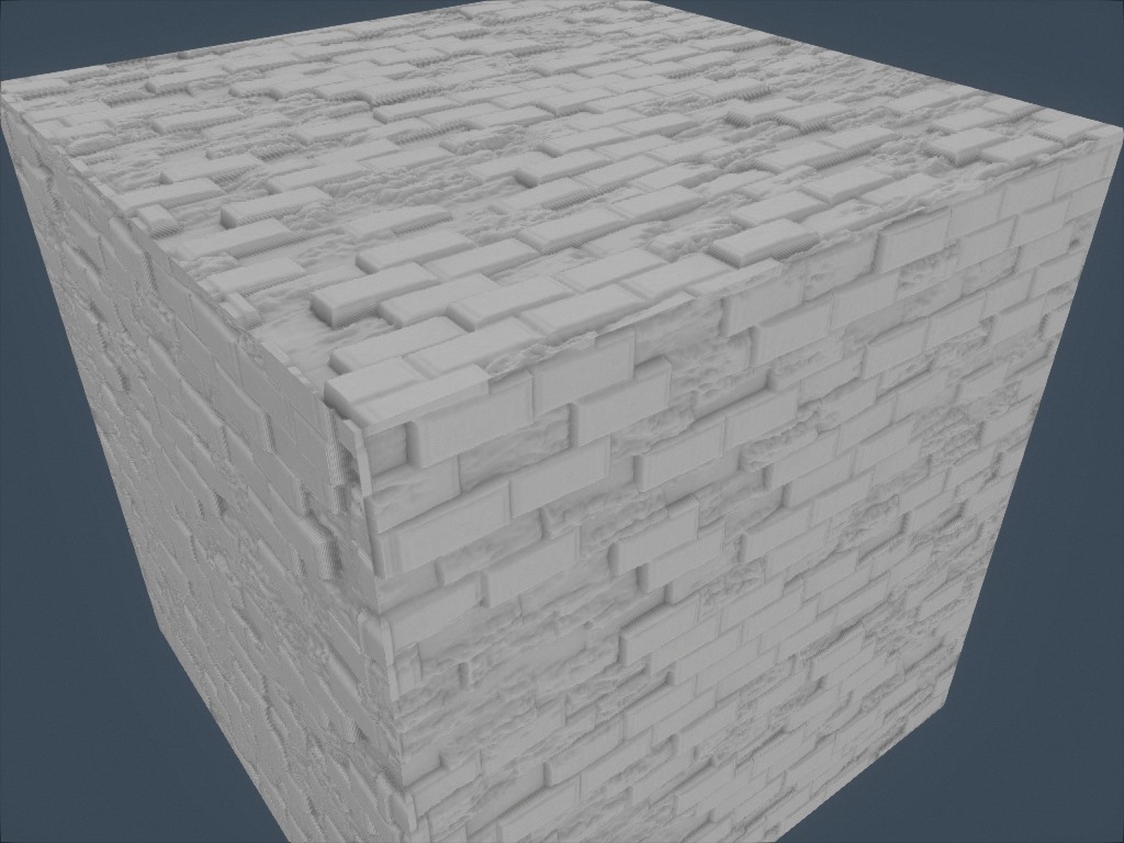
Growing Cubes
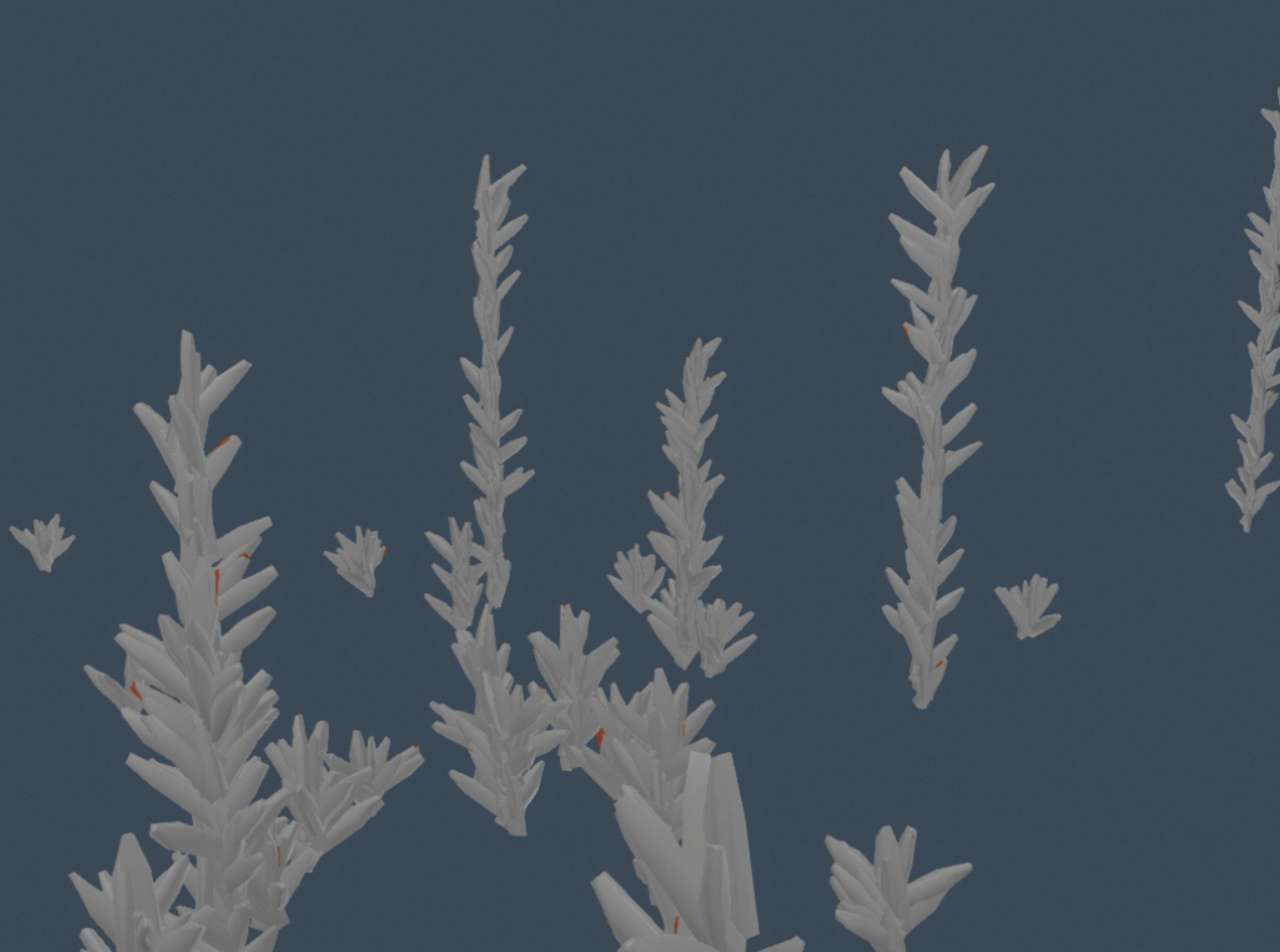
Combining and deforming simple cubes also has a lot of potential. For the vegetation in H – Immersion, we started from a cuboid, and deformed it a bit. Then we made many copies of the mesh placed vertically around an imaginary axis, with random size and orientation. This creates something that vaguely looks like a plant. We repeat, again with random parameters, to create more of them:
This looks very rough and you’re probably expecting to read what the next steps are to refine the shape. There aren’t any: this is the final mesh. We didn’t even create a custom texture for it. Instead, we just applied the ground texture on that mesh!
But during the demo, the effect works well enough thanks to the rendering, the lights and shadows, and a simple but convincing animation. The editing also helps a lot: the shapes and movements set the mood, but the viewer doesn’t have time to notice the details before the camera moves on. Sometimes evoking a shape with a proper mood is more effective than painstakingly modeling it.
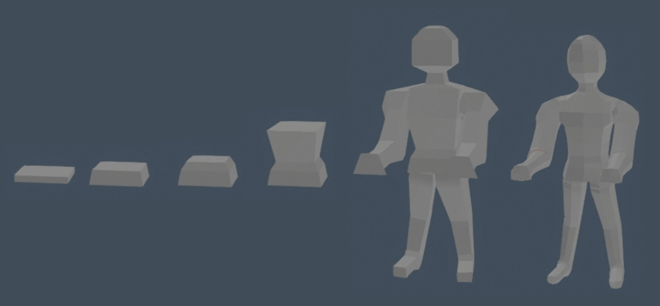
At some point, we wanted to have more complex meshes. As usual, we started from our beloved cube and decided to modify it. Merely deforming a cube will still result in.. well, a cuboid. So we needed something more. Enters extrusion: we pick a face, and extrude it. This operation will create a new face, which we can pull from the object, resize, or transform in any way we like.
We iterate multiple times, to create the shape we want. Each extrusion will add more details. The result is often low poly, but we use the Catmull-Clark subdivision algorithm to smooth the result out. This approach was inspired by the Qoob modeling tool.
What we’ve described is exactly what we did to generate the small statues used as decorating props in several places during the demo:
Since it’s all procedural generation, we can pass arguments to the function. These arguments can control some angles for the legs, arms, etc. Write a loop generating lots of statues with random parameters, et voilà! You have enough variation, so that it doesn’t get visually boring.
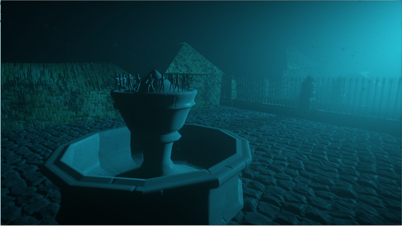
We also created two statues with hard-coded parameters, for better results. Here is how it looks after applying textures and lighting.
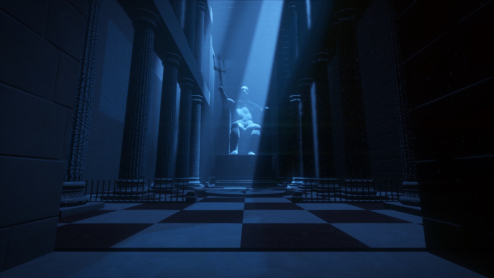
In the temple, we wanted to show a colossal statue of Poseidon seating on its throne. The technique used for the small statues was too rough for a model that would have more focus. Poseidon is huge and we wanted more details. The demo has a lot of content and fitting everything was a challenge. After a lot of size optimization work, we managed to get around one spare kilobyte. We decided to use it to get a better model for Poseidon.
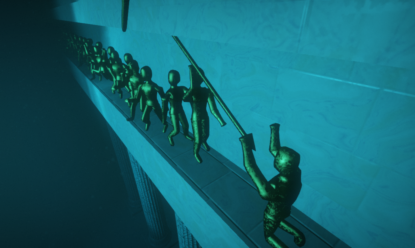
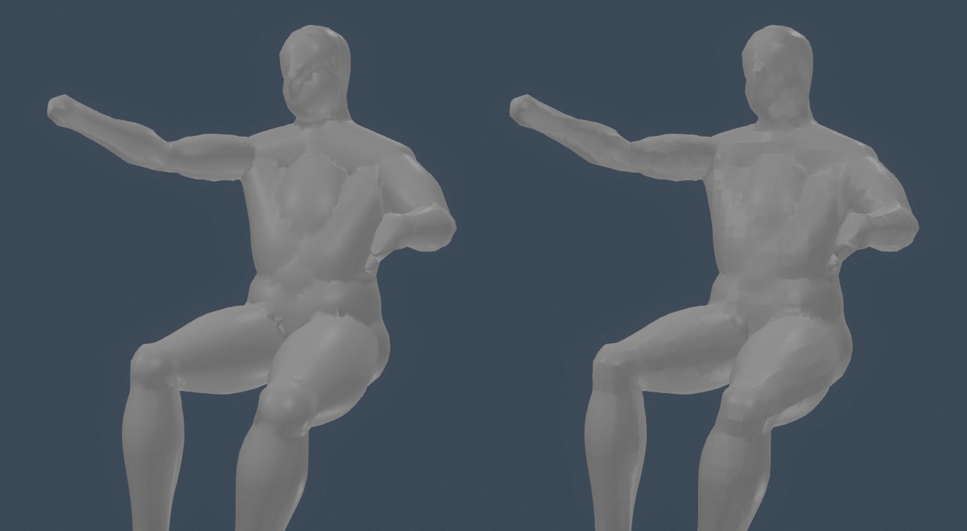
To do so, we used a completely different technique than what we’ve seen so far: implicit surface expressed with signed-distance fields (SDF). This is a technique very popular in 4kB intros, usually used with the ray marching algorithm to generate the result, and implemented as a screenspace shader. But since our rendering is based on meshes, we generated a polygon mesh by evaluating the SDF function with a marching cube algorithm instead of ray marching. We built the humanoid shape as a series of segments, with a little bit of tweaking to give it an organic look.
On the left, the normals deduced from the SDF reveal the underlying simple shapes. On the right, the normals estimated from the triangle mesh reveal the sampling grid, but hide the structure and give a desirable rough looking shape.
There was only so much detail we could afford, not to mention that modeling humans is difficult and people are very good at spotting issues in human-like models. We used to our advantage the low resolution of the generated mesh. It turns out that evaluating the normals on the final mesh (as opposed to deducing them from the SDF function) creates visible artifacts: the surface is full of smooth creases and edges. This very rough appearance can give sort of a sculpture look. We used lighting and cinematographic techniques on top of that to trick the viewer into filling the details. In the final shot, the statue seems more detailed than it actually is.
In creative activities, it is often crucial to iterate quickly on a design. You cannot do everything right from the first try, so you need to easily make changes, iterate, explore, see what works.
At some point, we put our mesh generator on a web server, just like we did with the textures. The webpage had a textarea where we could write C++ code. When we clicked on a button, it compiled the code on the server and returned the mesh in a JSON format. The webpage displayed the result with three.js, so that we could view and rotate the model with the mouse. Just like in Shadertoy, this allowed us to quickly try ideas, share them with the team, fork and tweak other models.
We later moved to a different solution, C++ recompilation, which we mentioned in the first part.
Conclusion
Mesh generation is arguably more difficult to design and more involved to implement than texture generation. When textures are just flat surfaces, meshes have different topologies, which adds a new layer of complexity.
But like with textures, the simplest building blocks can offer a wide range of possibilities to explore, as long as it’s possible to combine them in various ways. A few simple elements used creatively can give a wide range of shapes.
Moreover, as we’ve seen with at least two examples, the power of suggestion can play an important part and replace modeling work that would be tedious or even impossible to do with the available building blocks.
Using both of these observations can go a long way, as we hope to have demonstrated. The trick is to find the right balance between modeling work and expressiveness.
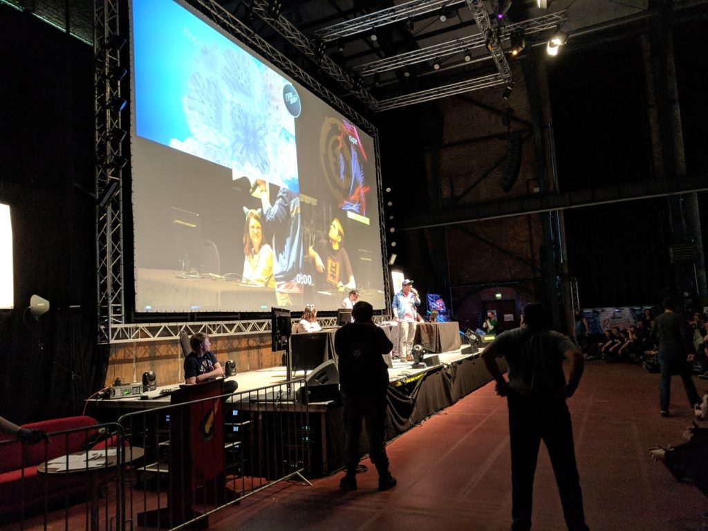
Earlier this month, the large demoscene Easter meeting, Revision, took place with all its range of events and competitions, despite a new online format due to the pandemic situation. One of those competitions is the Shader Showdown: a tournament where participants are to write the best possible visual effect within a limited time. Each round opposes two of them on stage for 25 minutes while a DJ is playing and the public is cheering. At the end of the round, the public decides the winner who moves up to the next round.
After this year’s competition, Friol interviewed six contestants, including the winners of the last three editions:
ferris is a software engineer coming from the US. He’s currently working on machine learning processors for Graphcore in Norway.
fizzer comes from the UK and is currently living in Finland. He is a graphics engineer who has been working on Cinema4D before doing GPU path tracing in Notch, a tool to create visual effects for events and concerts.
Flopine is a French PhD student in digital art and a technical artist at Dontnod. She won the Revision Shader Showdown 2020.
Gargaj is a Hungarian game developer. He has worked on the indie MMO Perpetuum before moving to the AAA industry with the Project CARS racing game series.
NuSan is a French technical artist who works in the game studio Dontnod and also creates small video games with Unity and PICO-8. He is the 2019 winner of the Revision Shader Showdown.
provod is a Russian software engineer from Siberia who recently moved to California and is currently working on the game platform Roblox. He won the Revision Shader Showdown in 2018.
For reasons we will not elaborate on, the original article was eventually withdrawn. With their permission, we’re sharing here their stories and insights for everyone to read.
What is this all about?
Whether it is at home, during a stream on Twitch, or as a performance during a live event, live coding consists in writing code with immediate visual feedback. In this article, it refers more specifically to writing a shader effect on stage to entertain an audience. At Revision and several other demoparties, participants have a given time to write their effect from scratch. A DJ is accompanying them with a live mix, and their code and its result are projected on a big screen for everyone to see, in a collaborative audio-visual performance.
When asked to define live coding, ferris mentioned a “competitive aspect which makes it at least e-sports like, while still being an inherently artistic medium”. Gargaj pointed out that “the shaders themselves are rarely rewatched afterwards”, unlike “a good demo that lasts years to come”. His comments emphasized the “in-the-moment performance”, comparing it to “rap or beatbox battles”. fizzer further described the “various twists and build-ups that occur during the coding session”, comparing it to the World Cup. “The end result does of course matter, but everyone shows up to watch the game in full because that’s where the excitement is”, he added.
This early video from 2011 can be a good introduction to shader live coding. It presents some simple 2D effects that are relatively accessible for a new programmer, compared to the 3D effects and advanced tricks seen in live coding competitions:
When did you first hear of live coding in the demoscene?
Flopine: When I entered Revision’s main Hall in 2016. I didn’t know it existed at all! That people would code live in front of others…
fizzer: I think it was when I read about IQ coding shaders as a member of Beautypi, which was a group that put on a show with live music and visuals. It wasn’t competitive, but it was live and I thought back then that it must be extremely difficult. It turned out of course that many years later it would be made an official competition at Revision and I found it to be quite fun when I tried it myself!
provod: At the demoparty WeCan 2013 in Poland. I was accidentally visiting this party (was visiting friends in Germany and became aware of a demoparty nearby) and only at the party place noticed that they had a live coding competition. A few years before that I had a rather small experience of doing music performances live coding PureData patches and live soldering custom digital synthesizers on stage, so that thrill looked like a lot of fun, even though I only began exploring shaders back then. So I just applied as a contestant and got selected. I’ve heard about live coding performances before that outside demoscene, mostly in the experimental electronic music scene. I always wanted to try doing something like that also with visuals myself, so I guess it felt like a good opportunity to just try.
ferris: In the form it is now, I guess 5+ years ago. I’m not sure exactly when. But I was aware of the first competition at WeCan (I think that’s where it was?) and I helped do some mac fixes for Bonzomatic in 2015 or so (which I think were superseded by more proper work by alkama etc) and I’ve tried to participate in most of the competitions that were happening at parties that I was attending around that time, especially as Solskogen was embracing them. That said, I remember there being compos with a similar format long before this. The “drunk master coding compo” comes to mind, which I never personally saw, but heard about from the likes of kusma / excess and a few others. I believe this was a feature of Kindergarden in Norway, but I’m not sure. This was more theme-focused, i.e. make a “texture mapped tunnel” and every time you hit compile you had to take a shot. Or something. :)
NuSan: I saw some people live coding sounds at local concerts. I also saw some live coding by IQ around 2012 on his youtube channel, but it’s really Revision 2018 live stream when I saw a proper shader showdown and that blew my mind.
fizzer: Actually I had never heard of live coding before I came across it in the demoscene. I had tried a few times to code something in a limited amount of time as a challenge for myself, such as coding an effect on a laptop during a train journey home, but I hadn’t ever imagined it as a real sport. I think it’s quite futuristic.
The editors
If live coding is a sport, the editor is its field, where the champions show their skills. Two shader live coding editors popular in the demoscene are ShaderToy and Bonzomatic. ShaderToy is a creative website where a community writes and shares shaders. It is a very nice place to find shaders and analyze how they are made. Bonzomatic is a software focusing on live shader competitions. Its author Gargaj shared the story behind the creation of Bonzomatic.
Gargaj: I know live coding has been a thing outside the scene since the mid-2000s, but I never really saw an appeal because the people doing it in “algoraves” were usually using very basic graphics or sound libraries. So the actual results were never particularly pleasant, and they were always somehow laced with an influence for either databending or 8-bit or both, which got really old after a while, and I never really saw the appeal.
The demoscene insertion happened when Bonzaj and Misz came up with the idea for WeCan 2013 and they created the competition using two projectors and a custom editor integrated into with Visual Studio; D.Fox (editor’s note: D.Fox is the lead organizer of Revision) liked the idea and tried to bring it to Revision 2014, but when it was announced (about a week or two before the party). I saw the package they were trying to use, which was really janky and obviously required extra hardware. Just to prove a point I found a Github repo by a guy called Sopyer that implemented a syntax highlighting editor over OpenGL, and within about 2 hours I had the basics for a tool that was able to show a shader that was being ran and recompiled. I then merged in some of Bonzaj’s code (like the FFT and MIDI code), and posted it back on Pouet. After the party itself, I was aware of the many bugs and the overall hacky nature of the editor, so I decided to write one from the ground up with a bit more thought and cleaner basics in mind. When I was looking for a name, I obviously thought of Bonzaj again and named it after him — something which he apparently never realized until years later.
A two hour long commented live coding session from NuSan using Bonzomatic.
When asked about the editor, the participants have all sorts of suggestions as to where to take it next. At a basic level, provod regrets the lack of a vi mode causing him to “feel crippled, and sometimes do slip live” while Flopine found its automatic indentation frustrating. To “keep the concept fresh”, fizzer suggests high level features like multipass shaders which “would allow a lot of unseen effects”, and mentions how a stateful shader would make effects “from basic feedback zoomers right up to physics and particle simulations” possible. These features became available in ShaderToy in 2016, enabling such effects.
NuSan was more interested in collaborative editing. The Cookie collective experimented that idea recently with a collaborative live coding where several coders were editing a shader simultaneously. Going further, fizzer wonders “what it would be like if the two contestants had access to each other’s shader output as an input texture”.
The heat of the competition
“I generally think that it doesn’t make sense to be alive and not constantly try to do the most complex and exhausting stuff in the dumbest way possible and with the silliest look.” — provod
The Revision 2018 final match: provod vs Flopine, with Ronny mixing.
Do you prepare for a live coding competition?
provod: Usually I do. I did not prepare for WeCan 2013 at all, however, and entered it at the party place on a whim really. It had a different format where you could continue to work on your shader in the next round, and in fact I immediately started making very specific preparations between rounds when I got the hang of it after the first round.
For subsequent compos I looked at participants list, got scared by all the big names, and decided that if I’m to at least show something comparable I should really have a few techniques memorized and should try to train myself to make a few scenes with these techniques combinations. I don’t do graphics professionally, and I’m not always involved with demoscene, so it’s not rare that there are a few consecutive months in which I don’t touch shaders (or any graphics stuff really) at all, so skills get very rusty. :D I certainly would not be able to write anything coherent if e.g. I forgot all the relevant math.
Usually a week or two before the compo I try to make a list of techniques to rehearse (e.g. raymarching basic loop, normals, basic shading) that I should be able to write with my eyes closed in a few minutes. Then I come up with a few scenes, maybe remember some ideas I had and did not have time to try previously. Then I just set up a timer and try a scene. Then I try to tweak a scene for a few hours to feel its “phase space” and get an idea what works and what doesn’t. Some of these end up being 4kB intros later :D.
NuSan: I try to train myself regularly by doing a shader coding live stream on Twitch each week so I have some pressure from an audience. Before an important showdown like the ones from Revision, I try to find an idea that could be original. A few hours before the match I mess around in Bonzomatic with that idea and try to find a nice visual target.
Flopine: I’m always prepared because I absolutely love coding shaders, thus I’m doing it all year long. And before a match or a VJ set, I usually practice and test ideas 2 hours before, until it’s my turn to go on stage! For the Revision showdown I often have 2 ideas at least, and then for the finals I’m always surprised and need to improvise more because I never think I’ll be able to pass the quarter and semi-finals!
Nusan: I don’t try to memorize each value or piece of code, it’s more about what steps I want to follow, so that once in the match I already know where to start and where to go. I don’t prepare for more than one round and usually there is at least an hour between two rounds so I can find a new idea. It’s a good process to get something cool on the screen without destroying all improvisation.
provod: I try to have at least three solid scene ideas each of which I can do within 20 minutes and tweak in the remaining minutes. There’s an interesting meta with these scenes, which scene I should play against whom and in which order. And I think I completely failed the meta for the past two Revision parties! It doesn’t mean that I have a super rigid scene idea for each round that I just type out (there were people doing this, I think, but my memory is way worse than that). Scene is mostly a vague pointer to a collection rendering techniques, geometries and maybe palette and camera movements. For some rounds I wasn’t sure what exactly I was doing before I started typing. And for some I just went and combined things from different scenes I practiced previously.
fizzer: When I know that I will be doing any kind of live coding, I brush up on basic flexible effects that I can code out quickly at the start. So during a round I will start with one of those and then just improvise on top of that. I think this is a nice compromise between going in cold and memorising an entire shader. Complete memorisation can be very risky. If it goes wrong, the time that it takes to come up with a Plan B can be significant. Likewise, if you have memorised some basic small effects that take little time to code then you have the choice of switching to another effect mid-round if it’s not going so well. You can also entertain the audience better that way, by making big changes to your shader mid-round.
What kind of shader will win over the audience?
Gargaj: That’s always a tough one, sometimes it’s just sheer visual splendor, sometimes it’s hitting the right note with the audience, sometimes it’s doing something more interesting than the other person even if it’s not as good looking. Plus there’s always audience bias as well :)
provod: Path tracing! It’s super trivial to do, and any random crap rendered with it looks good. It’s like pentatonic scale :D.
ferris: It depends on the audience of course. It’s the same with demos – people like what they like. For the demoscene, a cool 3D scene with lots of shiny things will often win. However, sometimes a very stylistic 2D shader will also win if it captures the audience (which is particularly common if it appeals to an “oldschool” palate, eg. by using a classic C64 color scheme/dithering style).
NuSan: Making some 2D neon lasers rotating in all directions always gives a good effect.
Flopine: The MirrorOctant from mercury sdf library! Such a cool way to duplicate space seamlessly. That function combined with a cool shape and maybe an angular repetition can win almost all shader showdown matches I’ve been into :) but I like to try different things because I don’t want to do stuff that are “too easy” on stage.
Flopine and Cupe look at each other’s creation after a match at Revision 2018.
Any particularly memorable live coding event?
NuSan: My first shader showdown in public (at Cookie demoparty) was very intense, my fingers were shaking but it was awesome. I had some bad live coding sessions mostly when I’m tired or if I do several sessions in a row. After a while, you can’t really think anymore and your creativity runs dry. Then it’s not fun and usually you lose ^^.
Flopine: The first time I went on stage at Revision 2018 will remain in my memory for decades I think! So exciting, so many emotions and fun… I think I want to feel that again over and over, that might be why I’m doing a lot of showdowns, but obviously (and unfortunately) the feelings are never as strong as they were the first time!
fizzer: A terrible one. It was Revision 2018. I had requested (or so I thought) to be coding in GLSL, but my computer on-stage had been set up for HLSL. This would ordinarily not be a huge problem, except that I didn’t notice this problem until some minutes into the round. I had no idea how to switch the shader language, and in my focused state of mind I had no choice but to continue, rewrite the code I had written in GLSL into HLSL and make the most of it. I still can’t believe that I was able to keep coding coherently after that!
provod: The whole Revision 2018 experience was completely surreal, I felt like such a huge impostor really. I was recovering from a severe flu (had been hospitalized just a few days before the party), so the preparation was interrupted, was sleep deprived due to long flights from Siberia, and also was desperately trying to finish a 4k and 8k before their deadlines. I did not expect to be able to write anything coherent on stage, even less so to win against all those strong sceners I still consider lightyears ahead of me.
Revision 2019 final, with NuSan and Flopine.
“Absolute panic”
On the third day of Revision 2020, a DJ set took place, together with another live coding event. Unlike the competition rounds, this session was much longer and not meant to be a competition, and more of a freestyle VJ. Accompanying Bullet during his mix, it featured not two, but three participants: Flopine, Gargaj, and IQ. IQ is widely known for having pioneered many ray marching techniques, creating the vegetation in Pixar’s film Brave, and being the coauthor of ShaderToy.
Gargaj talked about his reaction when he was asked to take part in the event.
Gargaj: Oh my first reaction was absolute panic when I found out at around 1:30AM that they want me in it too, and then just mounting anxiety. Then the whole thing kicked off and I just locked in to the keyboard and the screen. Aside from the quick HLSL-to-GLSL port, my focus narrowed in so much that I didn’t watch the stream, had no idea what the other two were doing, and completely forgot about the relaxo-beer I opened myself 10 seconds earlier. I don’t know if I’d call it “fun” to be honest, because while I was incredibly lucky that the idea I decided to go with worked out, it was really just luck and it could’ve been equally as much of a disaster with me staring at a blank screen for an hour. I really genuinely dislike things that have a time limit and try to actively avoid them. I got to participate (and let’s face it, totally undeservedly, compared to what others can do) against the two best people who do this, so it was at the very least a good entry on my demoscene CV. :) But I don’t know if I ever want to do it again.
The online event between Flopine, IQ, and Gargaj, with DJ Bullet, all streaming from different countries.
“It’s important to have fun during a match or else the pressure can be a pain.” — NuSan
Did live coding shaders get better with time, technically?
Flopine: For me I’m getting better each year, but not because I’m working on the same thing again and again. I’m learning new things every month and filling my own palette of techniques with them, which helps me build more complex/mastered images in my opinion.
In general, live coding shaders is also becoming better and better technically because intros and 4k are getting better and better! I once saw a path-traced shader typed under 25 minutes for a showdown! I think the demoscene and also papers that come out of research labs will continue to improve, thus improving what type of effect you can make in 25 minutes.
Gargaj: I don’t know, I don’t remember the first ones; if they’ve gotten better, I think it’s because people learned to scope the 25 minutes in better and started to explore more ideas.
NuSan: I think that live coding did get better, as new techniques are found regularly. Also there is a lot of knowledge sharing between demosceners so we can all improve, for example with shadertoy and live coding streams. Then some tricks might sometimes get lost, and also we are maybe too focused on technical skills and impressive shaders. We could spend more time on simpler but more improvised shaders that would be more personal and maybe fit the music better.
ferris: I think they’ve peaked a bit actually, and I think it has to do with a certain overlap of 1. what people can conceive of in their heads with such a limited format and 2. the round time limit. Admittedly I think it’s usually a bit stale, though we are seeing better and more impressive space folding/lighting stuff as GPUs get faster in particular. In fact I think GPU technology advancements are what drive live coding advancements more than coder skill, but it’s certainly not the only factor.
fizzer: I think they did. When the event was first introduced at Revision it was totally new. The idea of having the volume of the cheering from the audience dictate the winner in a very subjective manner was even more radical. It was quite hard to guess how it would work, and what the best strategy would be, how much stress it would be to code on stage in front of everyone. I think now it’s quite well established what makes a good live coding round and what to expect from it. It’s getting more intense every year, and some participants are effectively training all year round by doing time-limited live coding streams on Twitch in their own time, for example. I’ve been out of the game for a while, but I may yet return. We’ll see.
provod: Absolutely! My impression is that previously people generally were just improvising on the spot. But for the past year or two I see people both make special preparations for live coding compos (you can see that from the way people write complex scenes with great confidence) and keep themselves in good shape and are constantly refining their skills by doing shaders regularly. Like NuSan, evvvvil and Flopine streaming on Twitch (i’m sure there are other sceners who also stream shaders but I can’t remember them all). Unfortunately, I don’t have a time budget to keep a similar routine.
provod vs Ferris at Revision 2018.
Does live coding require distinct skills from coding?
Flopine: The demoscene is full of super great coders that don’t livecode! Live coding is stressful not only because you have to type and think fast, but also because you have to be present, to be on stage in front of hundreds of people that will judge both your production AND the code of it. I think a super talented coder needs to be sure every line is in its right place, that he does not implement something in a dull way or whatever… but in a live coding environment you don’t have time to think about all those!
ferris: Frankly I think the best coders are the ones that take their time and do something more comprehensive. live coding to me isn’t better/worse, it’s a very different thing, and it’s an odd skillset that to me doesn’t really overlap much with what I’ve typically thought of as “best” coding skills, though I have a lot of respect for it certainly!
NuSan: Live coding is a very special thing, focused around short and intense sessions. Also you have to sacrifice some elegance in coding style to get faster. Some coders prefer having time and peace of mind while creating and it doesn’t make them less impressive. Right now, I like live coding because it lets me create fast and I don’t have the patience to take my time.
provod: Yes. You have to be able to do a lot of stuff consistently in a very limited time and under quite a bit of pressure. Not everyone will find this fun. It is also laser focused on short-term results sacrificing everything else, so it’s kind of orthogonal or even outright adversarial to other code writing dimensions like code quality, performance, cleanliness etc, which are very important in real life, and lack of which would cause physical pain to many great coders I know.
provod vs NuSan at Revision 2019.
Who is the livecoder in the demoscene you appreciate the most?
fizzer: I would have to say Flopine, she has a real sense of showmanship and personality resulting in a real cool performance when she is live coding, and the shaders she produces are likewise always charming and funny. In the demoscene it was a bit like she came out of nowhere and suddenly started making these awesome live coding performances. She has also produced demos besides that too, and is very active online sharing her code and livestreaming on Twitch and such.
Gargaj: That’s a tough one; the NuSan / Evvvvil battle this friday was probably the most insane thing I’ve ever seen, and yet when you ask the question, I find myself thinking about people like Ferris and Cupe and Visy who usually do something completely lateral and non-3D, because I think that’s not only harder to pull off, but also shows guts. On a higher level though, what NuSan, Flopine, Evvvvil, yx, and the likes are doing with their weekly streams is fantastic and helps a great deal with community building and knowledge-sharing.
During the Revision 2020 quarterfinals, NuSan vs Evvvvil has been a memorable match.
provod: It feels weird to pick just one person — I envy all of them and would love to grow and be like them some day. Evvvvil is doing some crazy space warping stuff that I can’t wrap my head around. LJ is an absolute god of making complex (and realistic!) geometry. Nusan’s stuff is very beautiful and clean. And of course Flopine always comes up with some unconventional approach and kicks all of us default abstract raymarchers :D.
But if I absolutely had to pick one scener, it’d be Ferris. I love the diversity of the stuff he’s doing and the polish of it. And I absolutely hate the fact that he’s always ahead of me in whatever and is also doing it way better than I could ever event attempt (I wanted to do FPGAs, he’s already streaming it; I wanted to do some DJing, and he immediately streams a DJ set breakdown he did weeks earlier; etc. He’s also the person who showed me shaders in 2009 when I didn’t even know what those were.
Flopine: Tough question… I think I’ll always admire LJ, both for what he did in previous showdown tournaments and for the quality of his 4k. He gave me the initial spark not only because what he did was amazing but also because it “hit the spot” artistically, at least for me. The first time I saw him on stage I saw an artist, being in such control with his medium that he was capable of improvising a masterpiece on short notice. And then with his 4k I think he is also able to express a mood, a feeling and to share it with us. I’m very receptive to that and I’m glad to see more and more entries being sensible, like some from Primsbeing for example.
ferris: Admittedly, while I’ve tried to be somewhat involved in the live coding scene, as it’s become larger/more competitive, my interest has waned a bit. I’ve been in the scene for a long time and I appreciate the typical compo entries more, especially larger ones like 64k and full sized demos (even though I focused specifically on 4k’s in my late teens). When live coding happened, the fresh part for me was the spontaneity of it, that you could just bang out something and it would be cool. As people started memorizing more and more it was less interesting to watch, even though I know that’s not an easy feat and it’s impressive, it just doesn’t capture me personally as much. That said, blueberry is always my favorite person to watch because he comes up with crazy colors and usually fresh ideas, and I think he has a similarly not-so-competitive attitude as me. So, he’s both my favorite contestant and my favorite opponent :)
NuSan: Flopine often manages to surprise me with a new effect or style so watching her is a lot of fun. I also like coders who make impressive 2D effects, like Cupe or Ferris, it always feels magical to me.
Tomasz Bednarsz has been trying to increase the presence of demoscene at the major graphics community conference, SIGGRAPH, for a few years now, through so called “Birds of a Feather” sessions. This year I had the unexpected opportunity to attend SIGGRAPH in Vancouver, and I was invited to participate to the session along with a few other sceners. The details are available on the description that Tomasz posted.
There, I presented some aspects of 64k creation, that Laurent and I have been discussing here in the recent articles. The slides are available here:
A recording of the entire session is available. It includes the introduction by Tomasz, a presentation of a technique to render clouds in real time by Matt Swoboda (Smash, of Fairlight), our part, another take on 64k creation by Yohann Korndörfer (cupe of Mercury), and a presentation of Tokyo Demo Fest by Kentaro Oku (Kioku, of SystemK).
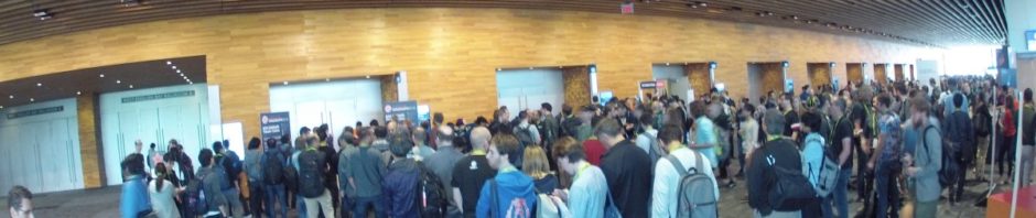
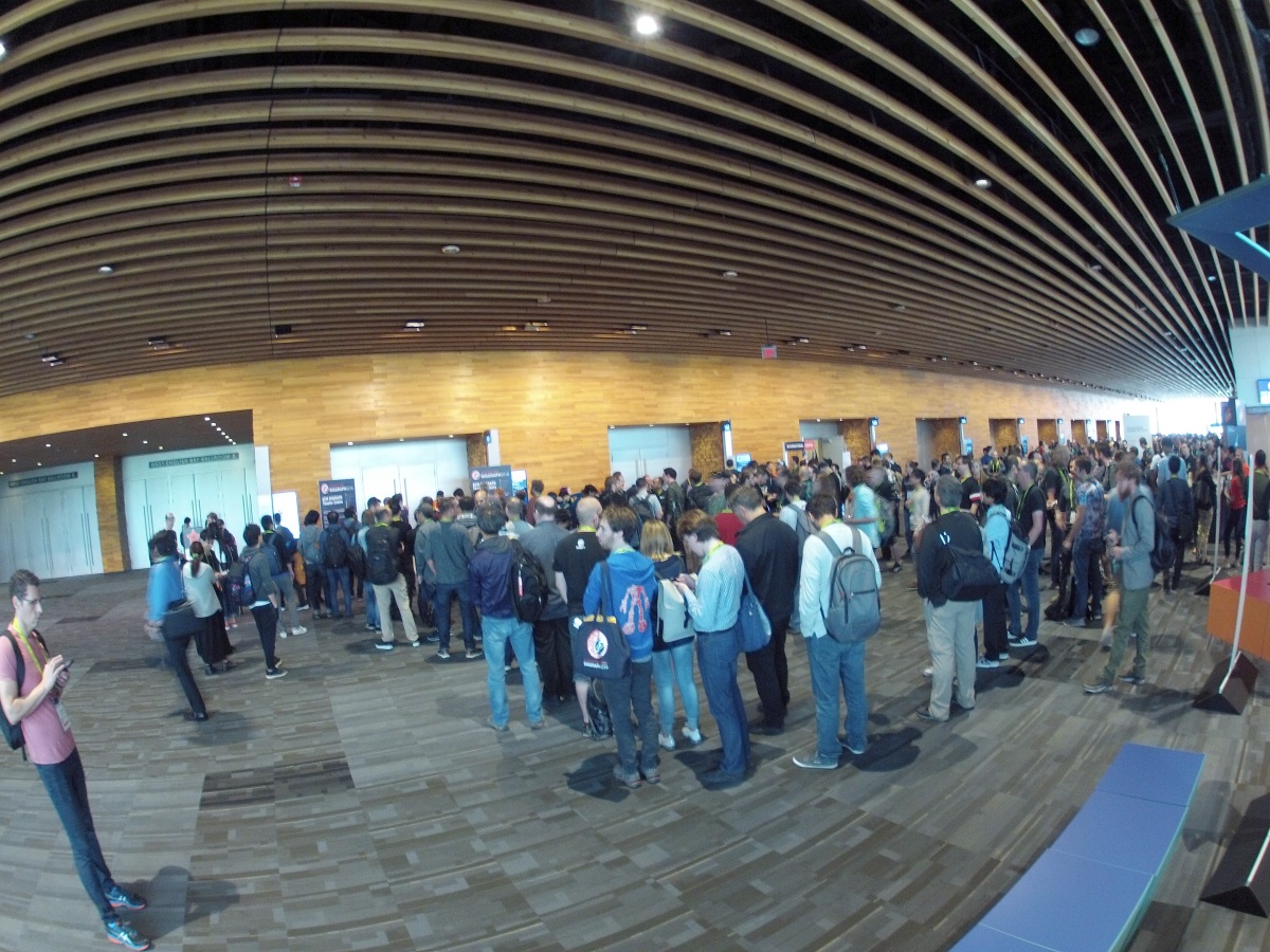
The event was way more successful than any of us expected, and we were all gladly surprised to see so much interest from the graphics community. A lot more people showed up than the room could accommodate, meaning that unfortunately most of them had to walk away.
The waiting line for the Birds of a Feather session on demoscene, at SIGGRAPH 2018.
Hopefully this increased interest means we can expect more events like this to happen at SIGGRAPH in the future years. We are already planning to do another demoscene session at SIGGRAPH Asia 2018, which will take place in Tokyo on December 4th to 7th.
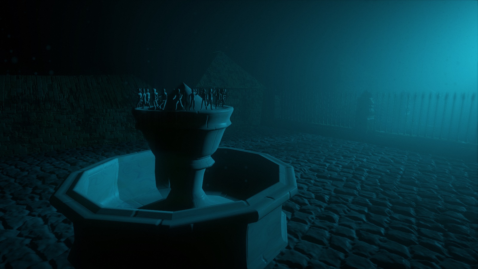
When making an animation within only 64kB, using images is tricky. We can’t store them in a traditional way, because it is not efficient enough, even with a compression like JPEG. An alternative solution is procedural generation. It consists in using code to describe how to create the images at runtime. Our implementation of such a solution is the texture generator, a core part of our toolchain. In this post we will present how we designed it and how we used it in H – Immersion.
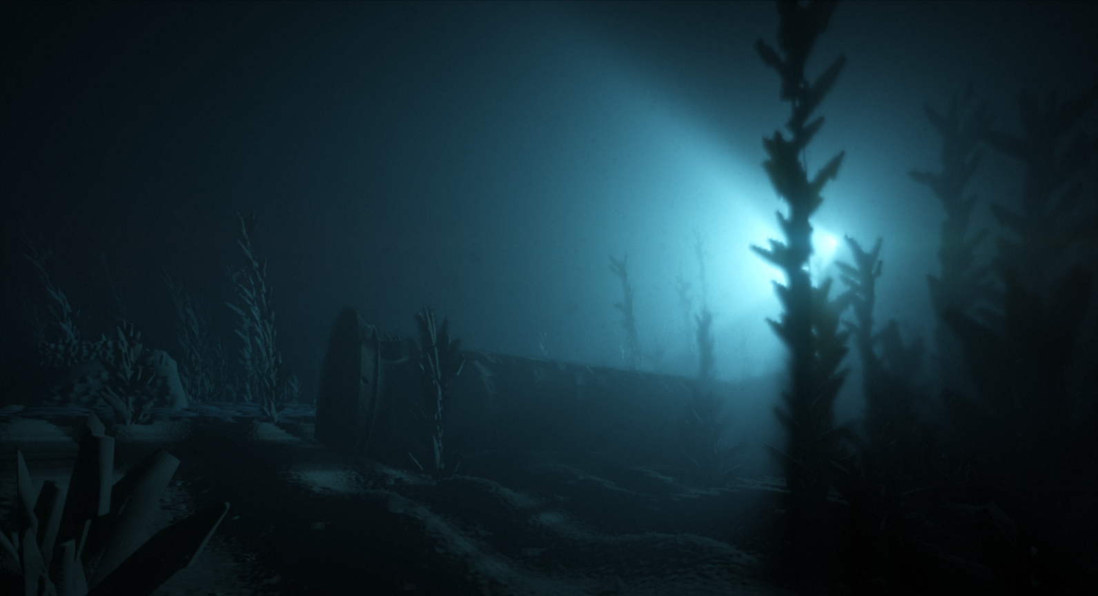
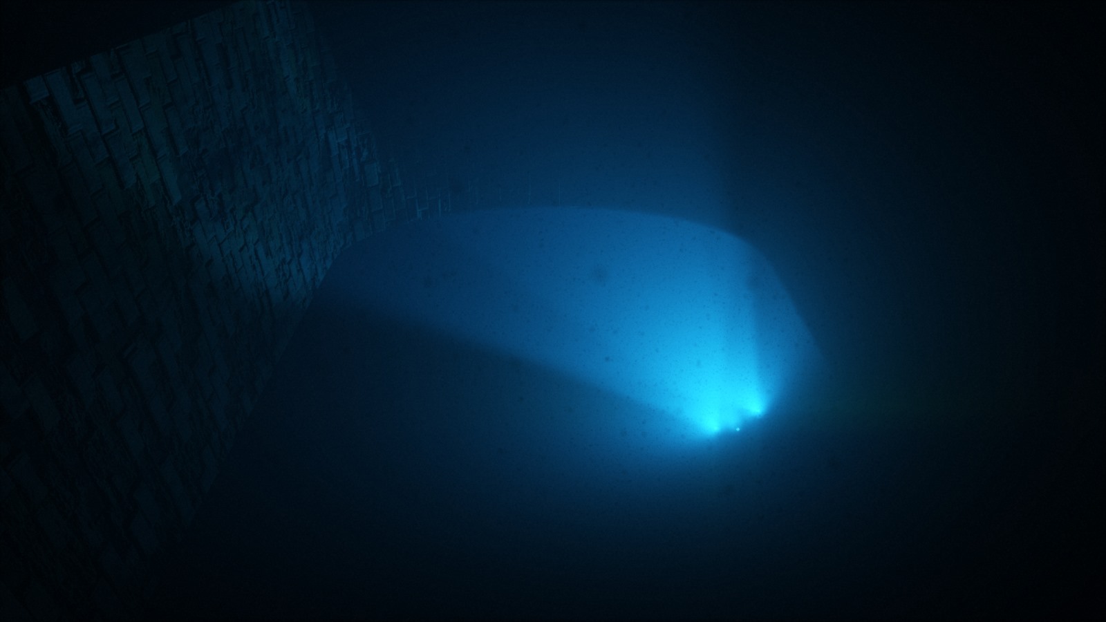
The spotlights of a submersible reveal details of the seafloor.
Early version
Texture generation has been one of the earliest elements of our code base: our first intro, B – Incubation, already had procedural textures. The code consisted in a set of functions to fill, filter, transform and combine textures, and one big loop to go over all the textures. Those functions were written in plain C++, but were later exposed with a C API so they could be evaluated by a C interpreter, PicoC. At the time, we were using PicoC in an effort to reduce iteration time: in this case it allowed to modify and reload the textures at runtime. Limiting ourselves to the C subset was a small price to pay for the ability to change code and see the result without having to quit, compile and reload the entire demo again.
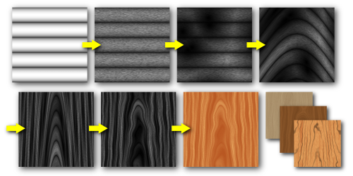
With a simple pattern, some noise and some deformation, we can obtain a stylized wood texture.
Various wood textures are used in this scene from F – Felix’s workshop.
We explored for a while what we could do with that generator, and ended up putting it on a web server with a small PHP script behind a simple web interface. We would write texture code in a text field, the script would feed it to the generator, which would then dump the result as a PNG file for the page to display. Soon enough, we found ourselves doodling from the office during lunch breaks and sharing our little creations among group members. This interaction was very motivating for creativity.
Our old texture generator web gallery. All the textures were editable in the browser.
A complete redesign
For a long time the texture generator almost didn’t change; we thought it was fine and our efficiency plateaued. Then we woke up one day, and discovered that Internet forums were suddenly full of artists showing off their 100% procedurally generated textures and challenging each other with themes. Procedural content used to be a demoscene thing, but Allegorithmic, ShaderToy and the likes had now made it accessible to the crowd while we had not been paying attention, and they were beating us hard. Unacceptable!
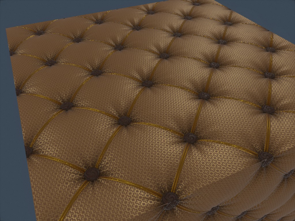
Fabric Couch
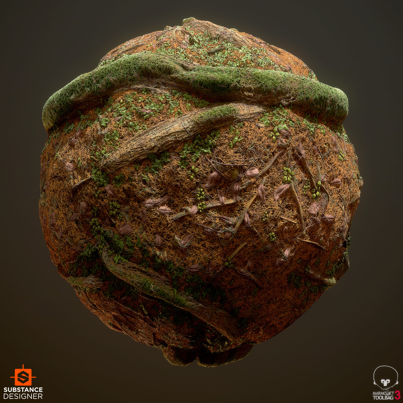
Forest Floor
It was long due time to reevaluate our tools. Fortunately working with the same texture generator for several years had given us time to understand its flaws. Our nascent mesh generator was also giving us some additional perspective on what we wanted a procedural content pipeline to look like.
The most important architecture mistake was the implementation of generation as a set of operations on textures objects. From a high level perspective, it may be a correct way of viewing it, but at the implementation level, having functions like texture.DoSomething() or Combine(textureA, textureB) has severe drawbacks.
First, the OOP style requires to declare those functions as part of the API, no matter how simple they are. This is a major problem because it doesn’t scale well and more importantly, it creates friction in the creation process. We don’t want to change the API every time we try something new. It makes experimentation more difficult, and ultimately limits artistic creativity.
Second, in terms of performance, it forces to loop over texture data as many times as there are operations. It wouldn’t matter too much if those operations were expensive relative to the cost of accessing large chunks of memory, however that’s usually not the case. Except for a few operations like generating a Perlin noise or doing a flood fill, most are in fact very simple and require few instructions per texture point. This means we keep traversing texture data to do trivial operations, which is ridiculously cache inefficient.
The new design addresses those issues with a simple reorganization of the logic. In practice, the majority of the functions just do the same operation for each element of the texture, independently. So instead of writing a function texture.DoSomething() which goes through all the elements, we can write texture.ApplyFunction(f) where f(element) only works on a single texture element. f(element) can then be written ad hoc for a specific texture.
This seems to be a minor modification. Yet doing so simplifies the API, makes the generation code more flexible and more expressive, is more cache friendly and trivially parallelizable. Many of you readers will probably recognize this as being essentially… a shader. Although the implementation is still, in fact, C++ code running on the CPU. We also keep the ability to do operations outside of the loop like before, but we only use that option when it is relevant, for example when doing a convolution.
Before:
// Logic is at the texture level.
// The API is bloated.
// The API is all there is.
// Generation of a texture has many passes.
class ProceduralTexture {
  void DoSomething(parameters) {
    for (int i = 0; i < size; ++i) {
      // Implementation details here.
      (*this)[i] = …
    }
  }
  void PerlinNoise(parameters) { … }
  void Voronoi(parameters) { … }
  void Filter(parameters) { … }
  void GenerateNormalMap() { … }
};

void GenerateSomeTexture(texture t) {
  t.PerlinNoise(someParameter);
  t.Filter(someOtherParameter);
  … // etc.
  t.GenerateNormalMap();
}
After:
// Logic is usually at the texture element level.
// The API is minimal.
// Operations are written as needed.
// Generation of a texture has a reduced number of passes.
class ProceduralTexture {
  void ApplyFunction(functionPointer f) {
    for (int i = 0; i < size; ++i) {
      // Implementation passed as a parameter.
      (*this)[i] = f((*this)[i]);
    }
  }
};

void GenerateNormalMap(ProceduralTexture t) { … }

void SomeTextureGenerationPass(void* out, PixelInfo in) {
  result = PerlinNoise(in);
  result = Filter(result);
  … // etc.
  *out = result;
}

void GenerateSomeTexture(texture t) {
  t.ApplyFunction(SomeTextureGenerationPass);
  GenerateNormalMap(t);
}
Parallelization
Generating textures takes time, and an obvious candidate for reducing that time is to have parallel code execution. At the very least, it is possible to generate several textures concurrently. This is what we did up to F – Felix’s workshop and it greatly reduced loading time.
However, doing so doesn’t shorten generation time where we most want it. Generating a single texture still takes as much time. That affects editing, when we keep reloading the same texture again and again between each modification. It is preferable to parallelize the inner texture generation code instead. Since the code now essentially consists in just one big function applied in a loop to each texel, parallelization becomes very simple and efficient. The cost of experimenting, tweaking and doodling is reduced, and that directly impacts creativity.
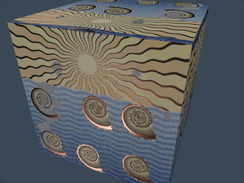
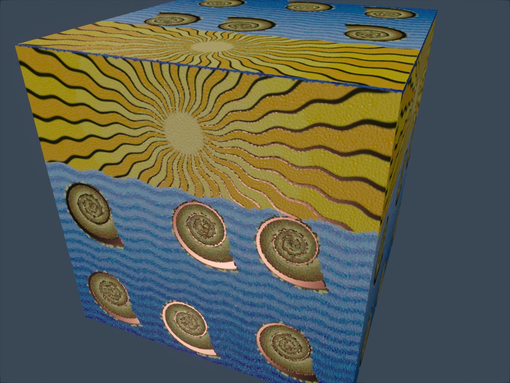
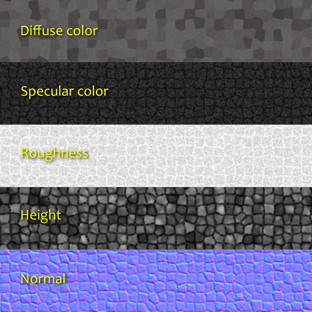
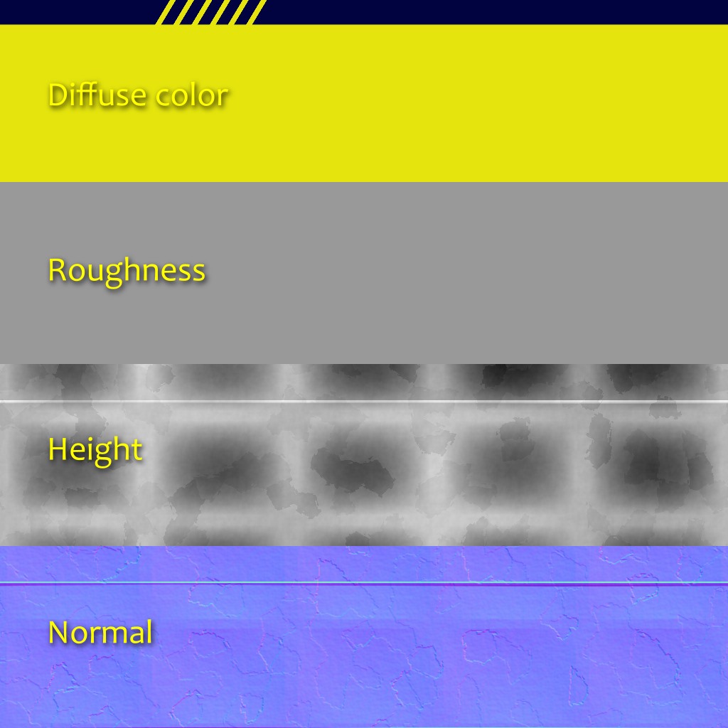
A damaged mosaic texture for H – Immersion
A mosaic texture for H – Immersion
This illustration is an idea that we explored and abandoned for H – Immersion: a mosaic decoration with orichalcum lining. It is shown here in our live editing tool.
GPU side generation
In case it isn’t completely clear in the paragraphs above, texture generation is done entirely on the CPU. At this point some of you might be staring at these lines with incredulity and thinking: “But, why?!”. Generating textures on the GPU would seem like the obvious thing to do. For starters it would likely speed up generation by an order of magnitude. So, why?
The main reason is that it was a smaller step of redesign to stay on CPU. Moving to GPU would have been more work. It would have required to solve additional problems, new problems we don’t have enough experience with yet. On CPU we had a good understanding of what we wanted and how to fix some of the earlier mistakes.
The good news however, is that with the new design it now seems fairly trivial to experiment with GPU side generation as well. In the future, testing combinations of both could be an interesting path to explore.
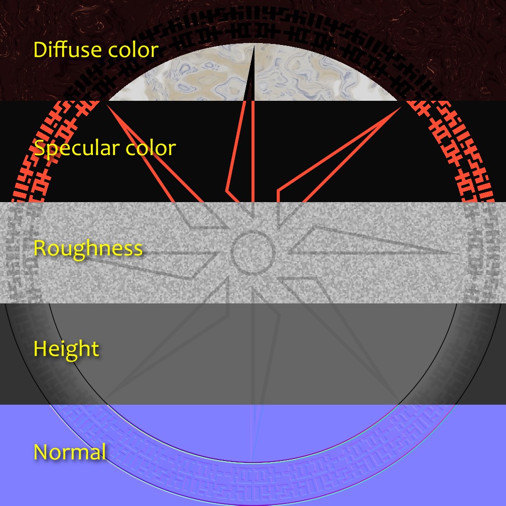
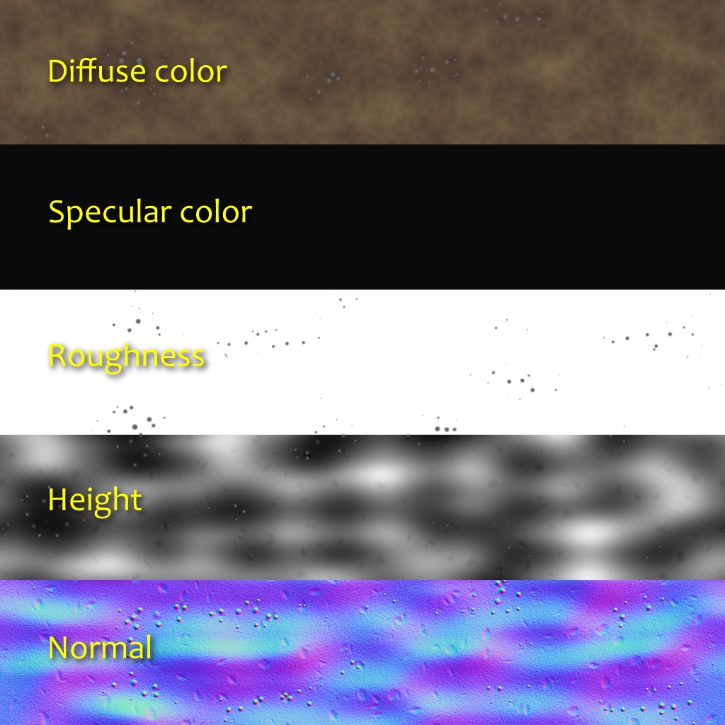
Texture generation and physically based shading
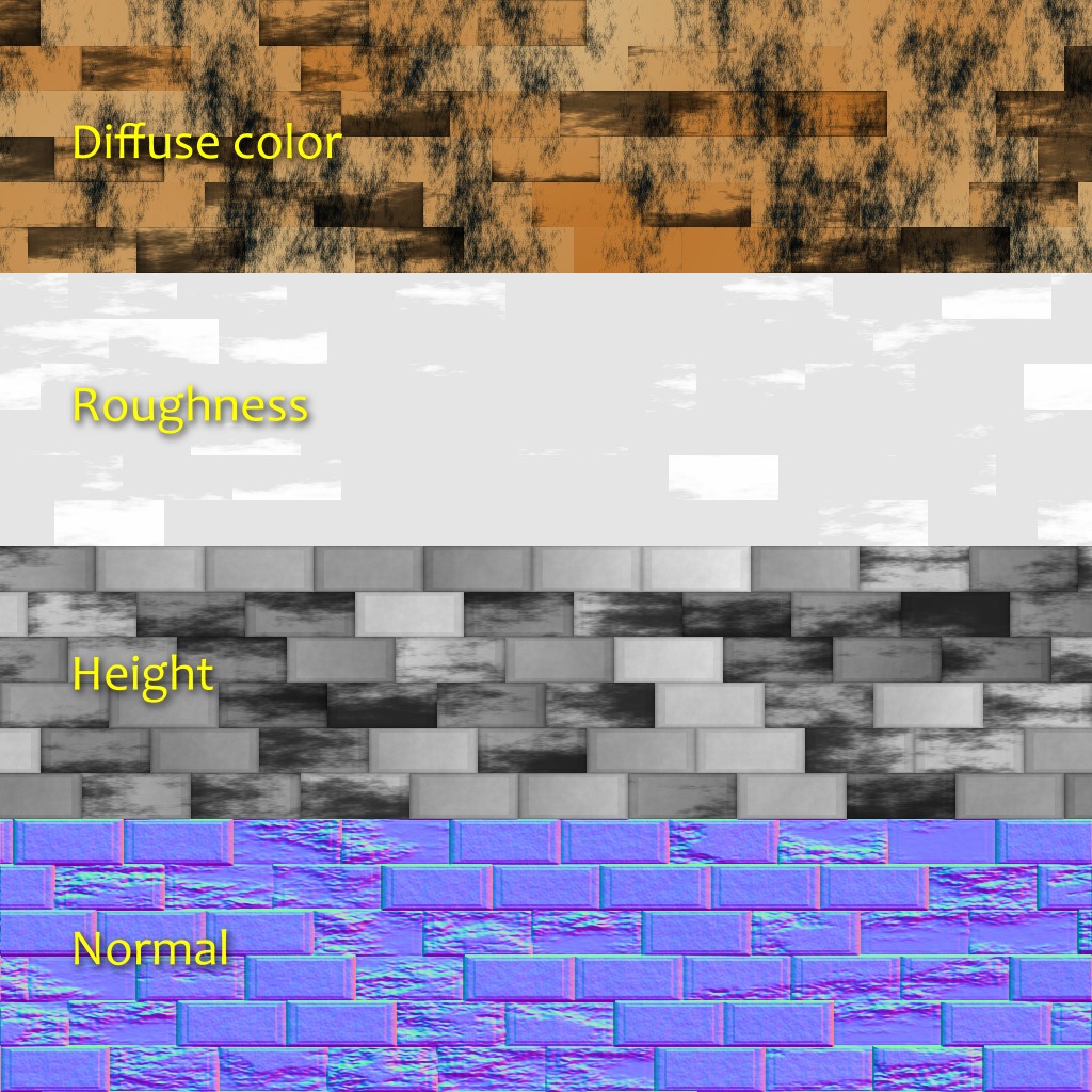
Another limitation of the old design was that a texture was considered to be just an RGB image. If we wanted to generate more information, say, a diffuse texture and a normal texture for a same surface, nothing was preventing us from doing that, but the API wasn’t actively helping either. This takes special importance in the context of Physically Based Shading (PBR).
In a traditional non-PBR pipeline, surfaces typically use color textures in which a lot of information is baked. Those textures often represent the final appearance of the surface: they already have some volume, the crevices are darkened, and they may even have some reflection highlights. If more than one texture is used at a time, it’s usually to combine details of large and small scale, to add normal mapping, or to represent how reflective the surface is.
In a PBR pipeline on the contrary, surfaces tend to use sets of different textures that represent physical values rather than a desired artistic result. The diffuse color texture, which is the closest to what we commonly describe as “the color” of a surface, typically looks flat and uninteresting. The specular color is dictated by the surface index of refraction. Most of the detail and variety come from the normal and the roughness textures (which you could argue represent the same thing, but at two different scales). How reflective the surface feels just becomes a consequence of the roughness. At this point, it makes sense not to think in terms of textures anymore, but in terms of materials.
Greetings marble floor texture breakoff
Cobbles textures breakoff
Fountain scene in H – Immersion
Seafloor textures breakoff
Seafloor scene in H – Immersion
Old stone textures breakoff
Arch scene in H – Immersion
Submersible body texture breakoff
Launch scene in H – Immersion
The current design allows to declare arbitrary pixel formats for textures. By making it part of the API, we can have all the boilerplate taken care of. Once the pixel format is declared, we can focus on writing the creative code, without spending additional effort on processing that data. Upon execution, it will generate several textures and upload them to the GPU, transparently.
Some PBR workflows don’t directly expose diffuse and specular colors, but instead a “base color” and a “metalness” parameter, which have some advantages and some disadvantages. In H – Immersion we use a diffuse+specular model, and a material usually consists of 5 layers:
Relief elevation (A; used for parallax occlusion mapping).
When it was used, emissive detail was added directly in the shader. It didn’t seem necessary to have ambient occlusion either since most scenes didn’t have ambient light at all. It wouldn’t be surprising to have such additional layers though, or other kind of information like anisotropy or opacity for example.
Wall texture without ambient occlusion
Wall texture with ambient occlusion
Pictured here is a recent experiment at generating local ambient occlusion based on the height. For each direction, march a given distance and keep the biggest tangent (height difference divided by distance). Finally, compute occlusion from the average tangent.
Limitations and future work
As you can see, the current design is a strong improvement over the previous one, and it provides creative expressivity. However, it still has limitations that we would like to address in the future.
For example, although it wasn’t a problem for this intro, we noticed that memory allocation could be an obstacle. The generation of a texture uses a single array of floats. For large textures with many layers, this can quickly hit the point where allocation fails. There are various ways to address this, but they all come with drawbacks. For example we could generate the textures tile by tile, which would scale better, but some operations like convolution would become less straightforward to implement.
Finally in this article despite using the word “material”, we have only talked about textures and never about shaders. Yet a material should arguably encompass the shading part as well. This contradiction reflects the limitation of our current design: texture generation and shading are two distinct parts, separated by a bridge. We have tried to make that bridge as simple to cross as possible, but what we really want is to treat the two as a whole. For example, if a material has static features as well as dynamic ones, we want to describe them in a same place. This is a difficult topic and we don’t know yet what could be a good solution but, let’s go one step at a time.
An experiment in trying to create a fabric texture similar to the earlier texture by Imadol Delgado.
Next up: meshes
Now that we’ve talked about textures, we invite you to keep reading to learn about mesh generation.
At last. Last December, we finally finished it. This video here is our last production, a 4 minute animation called “Immersion”. To be more precise, it’s a capture of what is usually referred to as a 64k intro. But more on that later.
Making it took the better part of two years’ free time. It all started during Revision 2015, a large event that takes place every year in Germany, during the Easter weekend. The both of us were chatting on our few kilometers long walk from the hotel to the party place, our faces battling the brisk morning air and the sleep deprivation. The previous night, the level of the 64kB competition had been high. Really high. The long established Hungarian group Conspiracy was finally back with a serious bombastic entry. Our best enemy Approximate was perfectly on time for its three years release cycle and showing a great deal of improvement in storytelling. The prolific Mercury now had a mature design style, with a foreshadowing intro title that left no doubt on the showdown.
That year, coming empty handed, we were not part of the competition, but we sure wanted to get back as soon as possible. Yet, after such a show we were wondering: slick look, great storytelling, great design… how could we get to that level? I couldn’t see what concept that, even perfectly executed, would have been a clear winner over any of those three. Not to mention that our tech was below any of them. And so there we were, throwing ideas on Hohenzollernstraße, when finally one of them stuck. A city rising out of the sea. That was a concept that, well executed, could maybe stand a chance at competing at the level this subset of that subculture had become. Revision 2016, get ready, here we come!
Revision 2016 zoomed past us with a whooshing sound… Revision 2017 it would be then. Alas, we barely made it to this new deadline either. At the party when people asked how it was going, the answer was a witty “It took us a year to make the first half, I’m confident we can make the second half in 24 hours”. We couldn’t. We did release though, but that second half was rushed, and it showed. So much so that we didn’t get even close to the podium. But we worked on it, gave it the love we thought it needed, and at last released the final version shown above.
What’s a 64k intro?
Demos are digital art creations at the crossroad of short films, music videos and video games. Although they present a non interactive experience, often music driven, like a music video does, they are rendered in real-time like video games are.
64kB intros, 64k for short, are like demos but with an added arbitrary limitation on the size: they must fit entirely within a single binary file of no more than 65536 bytes. No extra assets, no network, no extra libraries: the usual rule is that it should run on a freshly installed Windows PC with up to date drivers.
But how big is that exactly? Here are some comparison points.
In a 64kB file, you could store either:
400ms of wave sound with CD quality, or
3s of mp3 at 192kbps, or
A 200×100 RGB .bmp image, or
A JPEG picture of medium size, medium quality, like this 800×450 screenshot from the intro:
A 65595 bytes JPEG image, 59 bytes over the 64kB limit. :)
Yes, you’ve read that right: that video embedded at the beginning of this post, fits entirely within a single file that takes no more space than a just a screenshot from the video itself.
When you see these numbers, it seems complicated to fit in the binary all the images and sounds that surely must be necessary. We talked previously about some of the compromises we make and some of the tricks we use in order to make everything fit within such a small size. But that is not enough.
In fact, because of these extreme constraints, usual techniques and tools cannot be used. We wrote our own toolchain instead, a task that is an interesting challenge in itself: we create textures, 3D models, animations, camera paths, music, etc. thanks to algorithms, procedural generation and compression. We’ll talk about those very soon.
Some numbers
Here is an overview of how those 64kB are spent:
Music: 12.4kB
Meshes: 12.5kB
Textures: 4.8kB
Camera data: 1.3kB
Shaders: 6.2kB, from 5k lines of code
Engine: 12.9kB, from 20k lines of code
Intro itself: 12k lines of code
Time spent: hours, maybe over a thousand of them
This chart shows how the 64kB are used by the different type of content, after compression.
This chart shows how the binary size (excluding ~2kB of depacker) evolved until the final release.
Design & Inspiration
Having agreed that the central theme was a submerged city, one of the early questions was: how was this city going to look? Where was it located, why was it submerged, what was its architecture? One simple answer addressed all these points: it could be the legendary lost city of Atlantis itself. This would also explain and justify the emergence: by its divine nature (a literal deus ex machina). And thus it was so decided.
An early concept art for the emerged city. The artworks shown in this article were created by Benoît Molenda.
Two books guided our design decisions: Timaeus and Critias, in which Plato describes Atlantis and its fate. In Critias in particular, he details the structure of the city, its colors, its abundance of the precious orichalcum (which became an essential element in the temple scene), its circular shape, and the main temple dedicated to Poseidon and Cleito. Since Plato apparently based his description on countries he knew, a mix of Greek, Egyptian and Babylonian styles, we decided to stick with these.
Without proper knowledge of the topic though, creating convincing antique architecture seemed challenging. Instead, we decided to reproduce existing buildings:
The temple is essentially the Temple of Artemis at Ephesus, one of the Seven Wonders of the antique world.
Searching reference material for the Artemision turned out to be an unexpected, enriching experience. Originally, we were only looking for photographs, schemes or maps for reference. But when we learned about the name “John Turtle Wood”, things took a greater depth. Wood was the very person in charge of the searches and ultimate discovery of the temple location. Hoping that his name would yield better results than merely “Artemision”, we followed up, and we immediately found the book he wrote in 1877, in which he reports not only descriptions and drawings of the temple, but also his eleven years journey to find the lost site, his negotiations with the British Museum to stay funded, his relations with the local workers and the diplomacy involved before randomly digging holes.
Those books were essential to the design decision but above all, reading them brought us, as individuals, so much value from making this project.
And by the way, how is the roof supposed to look like? Some representations, including Wood’s, have a hole in it and some do not; there is apparently some controversy. We decided to go with an open roof model, allowing us to reveal the interior of the temple with a beam of light. The illustrations above show the floor plan and the cross sections, from the book Discoveries at Ephesus, compared to our work in progress model of the temple.
Achieving the desired look
We knew from the beginning that the appearance of water would be crucial to this intro. So we spent a lot of time on it, starting with watching reference material to understand the essential elements of underwater look. You might have guessed inspiration from James Cameron’s The Abyss and Titanic, 3DMark 11, or Ridley Scott’s Blade Runner for lighting.
Getting the right look wasn’t about implementing and turning on some epic MakeBeautifulWater() function. Instead, it was the combination of a series of effects that, when refined, would eventually trick us, the viewer, into accepting the illusion and feeling “This is it, we’re underwater!”. But one mistake, and the deception would collapse; a lesson we learned too late, when comments after the initial release pointed out where the illusion disappeared.
As illustrated above we also explored different non-realistic and sometimes extreme palettes, but we didn’t know how to achieve that look so we kept a classic color scheme in the end.
The water surface
The rendering of the water surface assumes a flat plane reflection. Reflection and refraction are first rendered to separate textures, using cameras on one side and the other of the water plane. In the main pass, the water surface is rendered as a mesh with a material that combines reflection and refraction based on the normal and the view vector. The trick is to offset the texture coordinates based on the water surface normal in screen space. This technique is classic and well documented.
It works well at a medium scale like during the boat scene, but at a larger scale like in the final emergence scene, the result looks artificial. To make it believable, an artistic trick we used was to apply a Gaussian blur to the intermediate textures. Blurring the refraction texture gives a murky look to the water, and a greater sense of depth. Blurring the reflection texture helps make the sea look more choppy. Moreover, applying more blur in the vertical direction imitates the vertical trails expected from a water surface.
A blurred image of the temple is reflected on the water surface.
The animation is done using simple Gerstner waves in the vertex shader, adding 8 of them with random directions and amplitude (within a given range). Smaller scale details are done in the fragment shader, including 16 more wave functions. A fake back-scattering effect based on normal and height brightens the tip of the waves, visible in the image above as small turquoise patches. During the launch scene, a few additional effects are added, like this rain drop shader.
Volumetric lighting
“How to make shafts of light for the submersible?” was one of the early technical questions. Maybe a translucent billboard with a beautiful shader could work? One day, we started experimenting with naive ray marching through a medium. We observed with delight that even in an early crude rendering test, and despite coder colors and the lack of a decent phase function, the volumetric lighting was immediately convincing. At that point, that initial billboard idea disappeared, never to be heard of ever again.
With this simple technique, effects we didn’t even dare think of where already baked in. As we added the phase function and played with it, it started to feel like the real deal. This opened a lot of possibilities from a cinematography point of view. But then there was performance.
Light shafts give this scene a look inspired by the film Blade Runner.
On each pixel, a ray is cast, and its intersections with each light cone are solved analytically.
The math is described here (now guess on what occasion the article was written in the first place ;-) ). In terms of performance, it would probably be more efficient to use a light volume bounding mesh, but for a 64k it sounded simpler to use an analytic approach. Obviously, rays only go as far as the depth in the depth buffer.
In case the ray intersects, the volume inside the cone is then ray marched.
The number of steps is limited for performance reason, and they are randomly offset to remove banding. This is a typical case of trading banding for noise, visually less questionable.
At each step, the shadow map corresponding to the light is fetched, and light contribution is accumulated according to a simple Henyey – Greenstein phase function.
Unlike epipolar coordinates based approaches, using this technique it is possible to have heterogeneous medium density, which adds more variety, but we didn’t implement such an effect.
The resulting image is upsampled using a two passes bilateral Gaussian filter and added on top of the main render buffer. Unlike Sébastien’s tutorial, we don’t use temporal reprojection; we just use a high enough number of steps to reduce visible artifacts (8 steps in low quality settings, 32 steps in high quality settings).
Volumetric lighting makes it possible to give a mood and a distinctive cinematic look that would be difficult otherwise.
Light absorption
An immediately recognizable aspect of an underwater image is absorption. As objects get distant, they become less and less visible, their colors fading into the background, until they disappear completely. Similarly, the volume affected by light sources is reduced as light is quickly absorbed by the water medium.
This effect has great potential for cinematography, and modelling it is simple. It is done with two steps in the shader. A first step applies a simple absorption function to the light intensity when accumulating the lights affecting an object, therefore modifying the light color and intensity when it reaches surfaces. A second step applies the same absorption function to the final color of the object itself, thus modifying the perceived color depending on the distance from the camera.
Test of light absorption in the water medium. Notice how color is affected by the distance from the camera and the distance from the light sources.
Adding vegetation
Seaweeds were an element we weren’t certain we could use. When reviewing the typical features of an underwater scenery, they were sitting among the top elements in the wish list, but their implementation seemed risky. Organic elements like that can be difficult to get right, and getting them wrong could break immersion. They would need to have a believable shape, be well integrated in their environment, and they might even require some subsurface scattering shading model.
One day though, we felt inspired to experiment. Starting from a cube, scaling it, and putting a random number of them on a spiral around an imaginary trunk: from far enough it could pass as a long plant with many small branches. After adding a lot of noise to deform the model it was already starting to look half decent.
A test shot with a few sparse plants.
However as we tried adding those plants to a scene, we realized the performance tanked rapidly with the number of objects. This limited way too much the number of them we could put for the image to look convincing. It turns out our new unoptimized engine was already hitting a first bottleneck. So we implemented a crude ad hoc frustum culling at the last minute (in the final version a proper culling is used :) ), allowing the dense bushes visible in the demo.
With appropriate density and sizes (patches with normal distribution), and the details taken care of by the dim lighting, it was starting to look interesting. Experimenting more, we tried to animate them: a noise function to modulate the intensity of an imaginary underwater stream, an inverse exponential function to make the plants bend, and a sinus so their tip would swirl in the stream. Doodling some more, we stumbled upon the money shot: the submersible casting a light through the bushes, drawing shadow patterns on the seafloor as it passed off camera.
The vegetation casting shadow patterns on the seafloor.
Giving volume with particles
Particles are the final subtle touch. Pay close attention to any real underwater footage and you will notice all sorts of suspended matter. Stop paying attention and it disappears. We tuned particles to be barely noticeable, preventing them from getting in the way. Yet they give a sense of volume filled with a tangible medium, and help sell the look.
The technical side is fairly straightforward: in Immersion, particles are just instanced quads with a translucent material. The rendering order problem due to translucency was simply avoided by setting the position along one axis according to the instance id. By doing so, they are always drawn in the correct order along that axis. The particles volume then just has to be oriented properly for each shot. In fact, in many shots this is not even done at all, since the size of the particles and the darkness of the scene made noticeable artifacts rare enough.
In this shot, particles provide depth cues and a sense of density as the submersible descends.
Music
How to fit a high-quality music in around 16kB? This problem is not new, and most 64kB intros written after .the .product in 2000 use the same concepts. The original series of articles is old, but still relevant: The Workings of FR-08’s Sound System.
In short, the idea is that we need the music sheet and a list of instruments. Each instrument is a function generating a sound procedurally (see for example Subtractive synthesis and Physical modelling synthesis). The music sheet represents the list of notes and effects to apply. It is stored in a format similar to midi, with some changes to reduce the size. During the execution of the program, the music is generated.
The synth has also a plugin version (VSTi) that the musician can use from his favorite tool. Once the music is composed, the musician clicks on a button, which will export all the data to a file. We embed the data in the demo.
When the demo is run, it starts a thread to generates the music in a giant buffer. The synth is CPU intensive and is not guaranteed to be real-time. This is why we start the thread before the beginning of the demo, while the textures and other data are generated.
Daniel Lindholm composed the music, using the synth 64klang created by Dominik Ries.
Workflow
Iteration time is one of the most critical aspects of the workflow when making a demo. In fact, this is true of many creative processes. Iteration time is king. The faster you can iterate, the more you can experiment, the more variations you can explore, the more you can refine your vision and increase the overall quality. So we want to eliminate as much as possible all the obstacles, all the pauses, all the little frictions in the creation process. Ideally, we want to be able to change anything, any time, and see the result immediately, as a continuous feedback while we are still making the change.
A possible solution, used by many demo groups, is to build an editor and create all the content inside the editor. We didn’t. Our initial approach was to write C++ code and do everything inside Visual C++. Over time, we developed a number of techniques to improve the workflow and reduce iteration time.
Hot reload all the data
If there was only one single advice to take away from this article, it would be this: make all your data hot reloadable. All of it. Make it so you can detect when the data is changed, load the new data when that happen, and update the state of your program accordingly.
One by one, we have made all our data hot loadable. The shaders, the camera, the editing, all the curves that depend on time, etc. In practice, we generally have an editor and the demo running on the side. Whenever we modify a file, the changes are immediately visible in the demo.
In a project as small as a demo this is fairly simple to implement. Our engine keeps track of where the data comes from, and a small function checks regularly if the timestamps of the corresponding files have changed. If they do, it triggers a reload of the corresponding data.
It might be significantly more involved in a bigger project where such changes are made difficult by complex dependencies and legacy design. But the impact it has on production cannot be overstated, so it is well worth the effort.
Tweakable values
Reloading data is all well and good, but what about the code itself? This is more complicated and we have approached this problem step by step.
The first step was a clever trick that allows to change the constant literals. Joel Davis described it in a post: a short macro that turns a constant into a variable with a piece of code that detects when the source file is modified, and updates the variable accordingly. Obviously in the final binary, this additional code is absent and only the constant is left. The compiler is therefore able to do all optimizations (for example when the constant is set to 0).
This trick is limited but it is really simple and can be integrated in the code in a matter of minutes. Moreover, although it is only meant to tweak constants, it can still be used for debugging purposes to modify a code path or toggle features with conditions like if(_TV(1)).
C++ recompilation
Finally our most recent update in our quest to make the code more malleable has been the inclusion of the tool Runtime Compiled C++ in our codebase. By compiling the code as a dynamic library and loading it, as well as doing a bit of serialization juggling, it allows to make changes to that code and see the result at runtime, without restarting the program or, in this case, the demo.
This is not perfect yet: the API is intrusive and constrains the design (classes have to derive from an interface), and compiling and reloading the code still take a few seconds. Yet the ability to make changes to the code logic inside the demo and see the result in situation enables a great deal of creativity. At the moment only our texture and mesh generators benefit from it, but in the future we want to extend it to the entirety of the “content” code.
To be continued
Here ends the first part of what will be a series of articles on the techniques used in H – Immersion. We’d like to thank Alan Wolfe for proof reading; you can check his many technical articles on his blog. In the next parts we will present in more details how the textures and the meshes are created.
Until then, feel free to ask any question or share your own experience.
When making a demo in 64kB (or less!), many unexpected issues arise. One issue is that sitting floating point numbers can take quite a lot of space in the binary file. Floats are found everywhere: position of objects in the world, position of the camera, constants for the effects, colors in the texture generator, etc. In practice, we often don’t need as much precision as offered by floats. Can we take advantage of that to pack more data in a smaller space?
In many cases, it’s not important if an object is 2.2 or 2.21 meters high. Our goal is to reduce the amount of space used by those numbers. A float takes 4 bytes (8 bytes for a double). The actual size on disk can be reduced a bit with compression, but when there are thousands of floats, it’s still quite big (compression doesn’t work well as the binary data looks quite random). We can do better.
A naïve solution
Suppose we have some numbers between 0 and 1000, and we need a precision of 0.1. We could store those numbers as integers between 0 and 10000 and then divide by 10. Whether we use 32 bit or 16 bit integers in the code doesn’t make a difference: since we don’t use their full range of values, all these integers start with leading 0s. The compression code will detect such repetitive 0s and use around 13 bits per number in both cases.
The problem with this solution is that we need to do some processing at runtime. Each time we use a number, we have to convert it to a float and divide it by 10. If all our data is in a same place, we can loop over it. But if we have numbers all over our code base, we’ll also need to call a processor in all those places. This simple operation can be cumbersome and expensive in terms of space.
It turns out we can get rid of the processing, and directly use floating point numbers.
A note on IEEE floats
Floats are stored using the IEEE 754 standard. Some of them have a binary representation that contains lots of 0 and compress better than others.
Let’s look at two examples using a binary representation. The IEEE representation is not exactly the same as in the example below (it has to store the exponent), but almost.
6.25 -> 110.01
6.3 -> 110.010011…
In fact, 6.3 has no exact representation in base 2: the number stored is an approximation, and it would require an infinite number of digits to represent 6.3. On the other hand, the binary representation for 6.25 is compact and exact.
If we’re optimizing for size, we should prefer numbers like 6.25, that have a compact binary representation. For example, 0.125, 0.5, 0.75, 0.875 have at most 3 digits in binary after the decimal mark. The binary representation will have a lot of 0s at the end of the number, which will compress really well. The great thing is that we don’t need processing code anymore because we’re still using standard floats. We just store normal floats, but we try to use floats that include lots of 0 bits and will compress well.
To better understand IEEE representation, try some tools to visualize the floats. You’ll see how removing the last 1s will reduce the precision.
How much precision do we need?
Floats are much more precise for values around 0. As our numbers get bigger, we’ll have less and less precision (or we’ll need more bits).
The table below is useful to check how much precision is needed. It tells you the worst error to expect based on the number of bits, and the scale of the input numbers. For example, if the input numbers are around 100 and we use 16 bits per float, the error will be at most 0.25. If we want the error to be less than 0.01, we need 21 bits per float.
Of course, each time you add a bit, you divide by two the expected error.
How to automate it?
An ad hoc solution is to remember this list of numbers and use them in the code when possible: 0.125, 0.25, 0.375, 0.5, 0.625, 0.75, 0.875. An alternative is to use a list of macros from Iñigo Quilez. As Iñigo points out, this is not very elegant. Fortunately, this is hardly a problem because chances are this is not where most of your data lies.
64kB can actually contain a lot of data. Developers often rely on tools and custom editors to quickly modify and iterate on the data. In that case, we can easily use code to truncate the floating point numbers as part of the process. If you use a tool to set the camera (instead of manually entering the position numbers), that tool could round the floats for you.
Here is the function we use to round the binary representation of the floats:
// roundb(f, 15) => keep 15 bits in the float, set the other bits to zero
float roundb(float f, int bits) {
  union { int i; float f; } num;

  bits = 32 - bits; // assuming sizeof(int) == sizeof(float) == 4
  num.f = f;
  num.i = num.i + (1 << (bits - 1)); // round instead of truncate
  num.i = num.i & (-1 << bits);
  return num.f;
}
Just pass the float, choose how many bits you want to keep, and you’ll get a new float that will compress much better. If you generate C++ code with that number, be careful when printing it (make sure you print it with enough decimals):
printf("%.10ff\n", roundb(myinput, 12));
The great thing about this function is that we decide exactly how much precision we want to keep. If we desperately need space at some point, we can try to reduce that number and see what happens.
By applying this technique, we’ve managed to save several kilobytes on our 64kB executable.
Hopefully you will, too.
People not familiar with the demoscene often ask us how it works. How is it possible that a 64kB file contain so much? It can seem magical, since a typical music compressed as mp3 can be 100 times as big as our animations – not to mention the graphics. People also ask why other programs or games are getting so big. In 1990, when games had to fit on one or two floppy disks, they used only 1 or 2MB (which is still 20 times as much as our 64kB intros). Modern games now use 10-100 GB.
The reason for that is simple: Software engineering is all about making trade-offs. The typical trade-off is to use more memory to improve performance. But when you write a program, there are many more dimensions to consider. If you optimize on one dimension, you might lose on the other fronts. We make optimizations and trade-offs that wouldn’t make any sense outside the demoscene.
First, we optimize all the data we store in the binary. We use JSON files during the development for convenience, but then we generate compact C++ files to embed in the binary. This saves us a few kilobytes. Is it worth doing it? If you had to make a demo without the 64kB limit, you wouldn’t waste time on this. You’d prefer the 70kB executable instead. It’s almost the same.
Then, we compress our file (kkrunchy for 64kB intros, crinkler for 4kB intros). Compression slows down the startup time and antivirus software may complain about the file. It’s generally not a good deal. I bet you’ll choose the 300kB file instead. It’s still small, right?
We use compiler optimizations that will slightly slow down the execution to save bytes. That’s not what most users want. We disable language features like C++ exceptions, we give up object oriented programming (no inheritance) and we avoid external libraries – including the STL. This is a bad trade-off for most developers, because this slows down the development. Instead of rewriting existing functions, you’ll prefer the 600kB file.
Our music is computed in real-time (more precisely, we start a separate thread that fills the audio buffer). This means that our musician has to use a special synth and cannot use his favorite instruments. That’s a huge constraint that very few musicians would accept outside the demoscene. They will send you a mp3 file instead. You also need a mp3 player, and your demo is now 10MB.
Similarly, we generate all textures procedurally. And all the 3D models. For that, we write code and this is a lot of work. This adds a huge constraint on what we do (but constraints are fun and make us more creative). While procedural texture have lots of benefits, your graphists will prefer using their normal tools. You get JPEG images and – even if you’re careful – your demo size increases to 20MB.
At this point, you may wonder if it makes sense to write your own engine. It’s hard, error-prone and other people probably made one better than you would. You could use an existing engine and it would add at least 50MB. Of course, it’s still a simple application made by a small team, you can imagine what happens when you scale this up to a full game studio.
So demosceners achieve very small executable sizes because we care deeply about it. In many regards, demoscene works are an art form. We make decisions meant to support the artistic traits we’re pursuing. In this case, we’re willing to give up development velocity, flexibility, loading time, and a lot of potential content to fit everything in 64kB. Is it worth it? No idea, but it’s a lot of fun. You should try it.
Our last production, E – Departure, is completely music driven and provides some fast camera moves. To make those visually more interesting we use a motion blur, that we happen to be fairly happy with. This article will be about explaining how this motion blur post processing effect is achieved. The shader language used in the code sample is GLSL.
E – Departure
Motion blur in real life
A photo with motion blur
First, let’s take a moment to remind what motion blur physically is. When a photo or a video is shot with a camera, the exposure time (or shutter speed) is a parameter commanding how long the film, or sensor, will be exposed to incoming light. The longer it will, the more light will be caught by the sensor, thus the lighter the image will get, and the more blurry moving elements will get. This can be seen as a drawback (in a dark environment having crisp images gets more difficult) or as a wanted effect (since motion blur conveys a sense of speed).
While the shutter is open, the effect of light on the sensor is more or less constant: all things being equal, a light trail should have a constant lightness. In other words, it’s almost a box filter. I feel this point needs to be stated since some people confuse this effect with the artistic mean consisting of giving more contrast at the base of the trail than at the tail. In photography such an effect can be achieved by firing a flash right before the diaphragm closes (a technique known as rear curtain sync), but this is not the kind of motion effect I am referring to in this article.
Velocity map based motion blur
I’d say there are mainly three ways of achieving motion blur: stochastic based, accumulative based and velocity map based.
The stochastic approach consists in randomly sampling at different points in time and doing a proper weighted average. Trivial in ray tracing, this is difficult to achieve with rasterization but there is research in that direction. Insufficient sampling will lead to noise.
The accumulative motion blur consists in imitating the physical effect by blending together snapshots taken over the duration of the simulated aperture. Doing so is expensive since for each frame the geometry has to be processed and shaded. Insufficient sampling will lead to banding.
The velocity map based motion blur consists in rendering one image of the scene, no different from the regular rendering one would have without blur, and to make every point of this image bleed in some direction according to its speed. To do so, the speed of each point is computed and stored in a buffer: the velocity map. This technique will have the same banding artifacts as the accumulative approach, and some more. This is the technique we chose.
Making three educated steps away from reality
Bleeding is not motion blur
At this point of the description, the velocity map technique is already expected to give a result that is not matching reality. The reason simply being that having object colors bleeding over each other is not equivalent to the accumulation of light during an aperture. Let’s give a simple example to illustrate this.
Viewer’s point of view
Imagine we have a black background, a static red sphere, and a moving white sphere passing in front of the red one. If the snapshot used for the final image is taken at the moment the white sphere is completely occluding the red one from the viewer point of view, the red sphere won’t contribute at all to the final image. With a camera taking a photo, there may be a part of the aperture duration when the red ball is still visible, hence contributing to the amount of light caught by the sensor. Accumulative motion blur will reproduce this effect while velocity map will not.
Expected resulting images
We know this is not accurate, but we are trading accuracy for speed, and as long as we don’t forget this and we accept the resulting quality this is ok. It is all a matter of balance between affordable and physically correct.
Linear motion versus arbitrary motion
Now another inaccuracy lies hidden in the velocity map technique description: the fact that we will make colors bleed in the direction of the speed. The wording suggests that the blur for a given point will always be linear. And this is what will be assumed, since it is way easier to store the representation of a linear move than any other kind of move. But then it means that points moving along a circle for instance, like with a rotation, will have a linear trail instead of a curved one. This approximation works as long as the amount of blur is supposed to be very limited compared to the path. But with elements making fast enough, like small circular moves, this will not work any more and glitches will become noticeable. Should this be a problem, I would suggest instead to store an instant center of rotation for example.
As long as we are using linear operations, we can also avoid computing the speed for each point, and instead just compute it for each vertex and interpolate between them. The benefit of doing so is obvious: the speed will be a varying value computed in the vertex shader, and available thereafter in the fragment shader.
Scatter versus gather
At last, let’s get even farther from reality for a technical reason, still trading accuracy for speed. As explained, we will have two images: a snapshot of the scene, and an image representing the speed of each point. Ideally, we would like to have each moving point bleed over its neighbors according to its speed. Unfortunately nowadays GPU are designed in a way so they can easily gather, but cannot scatter information: in a fragment shader, you can retrieve data from other fragments, but you cannot modify other fragments. So if you want to have one fragment affecting some other one, you have to read it from that fragment. And if you don’t know in advance which fragments are affected, which is the case here, for a given fragment you have to check all neighboring fragments and gather the ones affecting it. If a fragment might affect up to n fragments away, this mean having to check n² fragments, thus O(n²) (for more on this topic, see chapter 32 of the book GPU Gems 2). This quickly becomes very expensive.
So what we will do here is consider motion blur to be homogeneous enough so we can trade the scattering we would like to do for a simple gather operation. Instead of making our fragment bleed over, we will dilute it among other fragments. This is a strong assumption, that will often prove false. But fortunately, the average result will still look nice, even though some obvious artifacts will appear here and there.
Computing the velocity map
Let’s now get to the implementation part. I am supposing here we have some FBO (Frame Buffer Objects) ready, in order to be able to have efficient render to texture, or the equivalent if the API is not OpenGL. I won’t go into further details about this since it is quite a different topic from what is being discussed here. If you don’t know how to set up and use FBO, at least you now have the keywords and can Google it.
We will need a couple of things to build our velocity map. First we will need a separate buffer to store it. With OpenGL this is done with glDrawBuffers(), which allows to tell which buffers we are going to writen into. By default there is only one such buffer, but we can have various of them; here we just need an additional one. Second we will also need a way to compute the speed of the vertices. The motion blur is a screen space effect, so all we need is the speed in screen space.
During a typical forward rendering pass, each object will have some kind of matrice, pile of matrices, or any equivalent mean to compute its position in world coordinates. The camera is likely to have its own set of matrices, to transform points from world space to camera space, then from camera space to screen space (in OpenGL this last transformation is typically defined by the matrix referred by GL_PROJECTION_MATRIX). The position of a vertex at the given time t is therefore multiplied by each of those matrices to get the final position in screen space. To know the speed of such a vertex in screen space, we just need to know where it was at the time t – dt. If dt is exactly the duration of the aperture, the two positions will define the limits of the motion during that time. This is exactly what we want.
So basically we need a way to retrieve the transformation at t – dt while rendering at t. Using an animation, this shouldn’t be too difficult: you just have to query your system for t – dt. If your animation is ad hoc, like with some real-time interaction, then you may store the previous transformations. Anyway, as long as you have both the previous object transformation position and the previous camera position transformation, you have it all.
In a minimalistic vertex shader, one would have something like the following:
void main() {
  gl_Position = gl_ProjectionModelViewMatrix * gl_Vertex; // equivalent to ftransform(), which is a deprecated function
}
For each object we will feed the shading pipeline with an additional information: the transformation matrix of t – dt. I considered that the projection matrix was unlikely to change fast enough to have any consequence on motion blur, so I decided not to store it, and to use the current one for both the old and the current position. It is up to you to choose your policy, but you have to be consistent when computing the speed in the end. Anyway, this leads to the following new vertex shader:
You may notice that the current position is computed twice (gl_Position and newScreenCoord). I let it this way to make the code easier to read, since it seems the shader compiler will optimize this anyway. Also, you have to be careful about the homogeneous coordinates operation.
From now on let’s retrieve the interpolated speed in the fragment shader and finally store it in the velocity map. A typical fragment shader would look like this:
void main() {
  gl_FragColor = /* whatever */
}
We are simply modifying it the following way:
varying vec2 speed;
vec3 getSpeedColor() {
  return vec3(0.5 + 0.5 * speed, 0.);
}

void main() {
  gl_FragData[0] = /* whatever the fragment color was */
  gl_FragData[1] = getSpeedColor();
}
This is it. At this point we have a velocity map where color represents the motion of each point in screen space. So far so good.
Update: Actually, so far, not so good. The above code contains a bug that I didn’t notice at the time because we rarely met the conditions to make it visible. But since then it has been bugging me as we have been working on a scene that exhibits it pretty badly.
When polygons get clipped, it may lead to broken speed values, resulting in annoying strong blur artifacts. The reason behind this is the non linear operation consisting in dividing by the w component in the vertex shader, that brings wrong values after clipping.
To solve this, I suggest not dividing in the vertex shader and pass the w component to the fragment shader in order to divide only at that time.
Using the velocity map and applying the blur
Once the color buffer and velocity map are filled, the post processing pass will use both to generate the motion blurred image. This is done very simply: while in a very minimal blitting shader you would have something like the following,
In this example, the inc value will define a 10 fetches motion blur. It proved to be sufficient in our case, and even as little as 8 fetches could be enough for moderated blur. With 20 fetches it becomes really hard to notice artifacts, but it is also slower of course.
The function argument intensity controls the length of the motion trails. You can set it to be consistent with your rendering speed, or low for a fainter effect, of high for an exaggerated effect.
Dealing with precision matter
At this point, I had a nice looking motion blur already, but I noticed it tended to introduce instability at low speeds. This is due to the fact that low speed means short velocity vector, which being stored with two integers loses precision both in speed and direction. To overcome this issue, I decided to represent differently the velocity vector.
First, instead of storing its components, I stored the components of the normalized velocity vector on one side, and the norm on the other side. This dealt with the direction problem.
Second, I applied the very same trick gamma correction relies onto: using the power function to increase the precision of low values, at the cost of precision for high values. The norm would then be stored in non linear space, and transformed back when using it. Since varyings are interpolated linearly, we have no choice but stay in linear space in the vertex shader, and change for non linear space only in the fragment shader.
So in the vertex shader, once we have our per vertex speed vector we store it this way:
Update: again, for the reason mentioned above, this code has to be changed and norm has to be computed in the fragment shader. I am too lazy to fix the code here so this is let as an exercise to the reader. ;-)
Bugs and limitations
Motion blur artifacts
Just like said, each trade off introduces inaccuracies, that result in visual artifacts. The most important one is obviously the scatter vs gather one. You can see the visual cost implied here: notice the ghost effect visible on the edge of some elements.
Another problem is how to manage the edges of the image. When an object is moving near the border, the algorithm may try to fetch colors outside the image. In that case, I see three solutions: leaving it as is if this is fine in your case (it might simply not happen often enough to be a problem), clamping the fetch to the border (this is what is done in E – Departure; notice how it affects the right side of the sample screenshot), or generating a bigger image to have a thin space outside the displayed frame where colors can still be fetched.
Those problems though are difficult to notice at low speed, and will appear only briefly at higher speed. So for E – Departure, this was an acceptable trade off.
Conclusion
I presented here a technique fairly simple to implement, allowing to get an effect which is visually pleasing, and that noticeably increases the realism of the image for a limited cost. It played an important role in our demo; I hope you will find a good use for it too.