How do demosceners create complex computer animations in just a few kilobytes? One of our secret weapons is Shader Minifier, a tool that minifies GLSL code. Over the years, it has evolved to pack more data into tiny executables, pushing the boundaries of what’s possible. In this blog post, we’ll go through its evolution.
In 2010, I noticed a trend in the demoscene: creators were producing impressive 4k intros, but the process was incredibly manual and tedious. These intros relied on shader code to generate graphics, and optimizing this code was like a code golf competition. As the existing tooling was poor, I decided to help. My goal was to automate the most boring tasks: removing unnecessary spaces and comments, and renaming variables to a single letter. This is how Shader Minifier was born.
The compression paradox
One of the first features I implemented was the insertion of preprocessor macros. This is a classic trick often used in code golf competitions and obfuscation contests:
#define R return
By adding this line at the top of your code, you can replace every instance of “return” with “R”, saving 5 bytes per statement. This can quickly add up, especially if you apply it to other common keywords or standard function calls.
But someone once asked me: “Shader Minifier makes files small, but how many bytes does it actually save after compression with Crinkler?” Crinkler is the most popular compression tool for small intros.
At first, I didn’t care much: if I make the code smaller, the compressed code will obviously get smaller too… right? Nope, I was wrong. I tested it and I found out that the output of Shader Minifier was compressing to something bigger than the non-minified code. Was it bad luck? I experimented and adjusted some heuristics in the code. Is it best to introduce more macros or fewer? After multiple iterations, I found that the best approach was… to do nothing. Do not replace code with macros.
Turns out, Crinkler is smarter than I thought, and my clever macros were getting in its way. Modern compressors are excellent at identifying redundant patterns. If the word “return” is repeated throughout the code, the compressor can handle it very efficiently. Using macros to eliminate these redundancies is counterproductive.
Renaming: not as easy as ABC
Renaming identifiers seems like an obvious feature for a minifier. Initially, the goal seemed simple: use a single letter for each identifier. After all, one letter per identifier is optimal, right? Yet again, I was mistaken. Not all letters are equal when it comes to compression.
A good name is one that you reuse. If multiple variables have the same name, the code will look more repetitive and compress better.
So our strategy is to be pretty aggressive in reusing names:
- Variables in two different functions can obviously use the same name.
- If a global variable is not referenced within a function, we can also reuse its name thanks to variable shadowing.
- We can even reuse function names. With function overloading, the compiler will distinguish them as long as they have different arguments.
Yep. We’ve been so aggressive in reusing names that we’ve discovered bugs in glslang:
- https://github.com/laurentlb/shader-minifier/issues/435
- https://github.com/KhronosGroup/glslang/issues/3931
When a minifier breaks your compiler, you know you’re pushing boundaries.
Reducing the number of unique variable names is very effective. But you also have to pick good names. Should we name the variable “V” or “A”? Experiments show that picking one name or the other can affect the compressed size. It’s hard to know which name will perform better, but we compute the frequencies of letters and bigrams to guess which names are more likely to be better. The idea is to look at which characters appear more often in the rest of the code, and which pairs of characters are already common. In the end, it’s just a heuristic, and we could probably do better.
8k is bigger than 4k
With these features implemented, my original goal was achieved. Many demosceners have been using Shader Minifier for years to create their mind-blowing 4k intros.
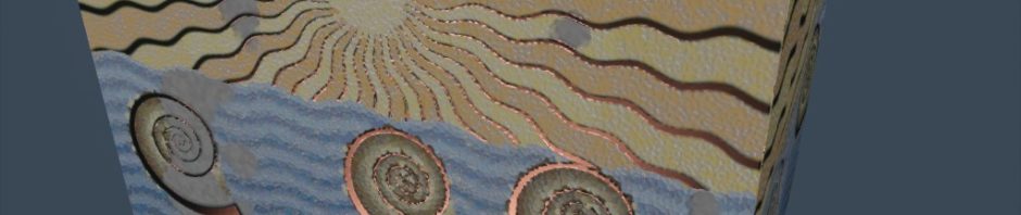
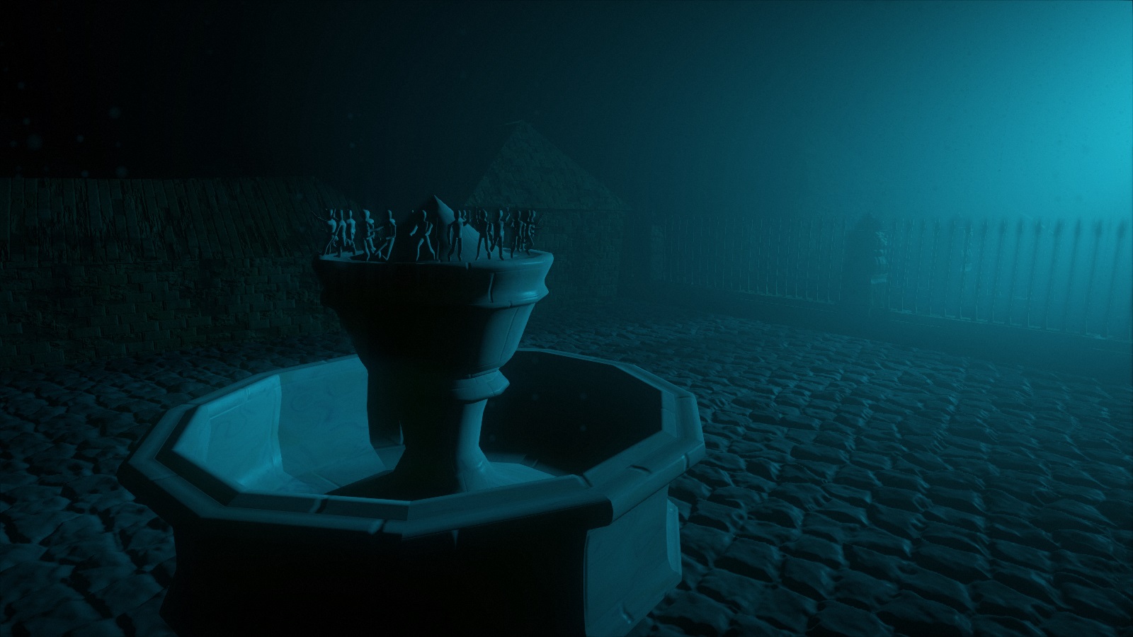
But one day, I decided to create my first 8k intro. The story behind The Sheep and the Flower was detailed in the blog post “How we made an animated movie in 8kB”.
Size-coding and code golfing are fun when there’s a small amount of code. But as the codebase grows beyond 1,000 lines, micro-optimizations become increasingly painful. The problem is that we also need to maintain and iterate on the code, so it needs to remain readable throughout the development of the intro. To be able to sheep my intro, more features were needed in Shader Minifier.
Here’s a graph showing the evolution:
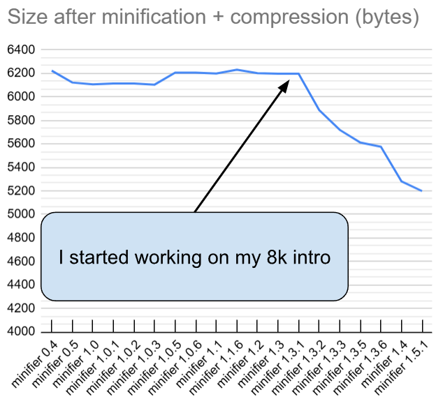
This graph shows the evolution of Shader Minifier and how big my 47kB shader code will get after minification plus compression. Without minification, Crinkler compresses the code down to about 10kB. I compared around 20 different versions of Shader Minifier and compressed their output with Crinkler to track the tool’s evolution.
So the recent improvements to Shader Minifier have saved about 1kB on this specific shader (between version 1.3 and 1.5). But don’t focus too much on this number: some of the improvements are about quality-of-life, not raw size. For example, it’s nice that we no longer have to manually find and remove unused functions.
In case you wonder about the size regression in version 1.0.5: at that time, we lacked proper tests for compression, so it went unnoticed (it was something related to renaming heuristics). Testing infrastructure is something that we improved later. Anyway, the point is that 47kB became 5.2kB after minifier and compression magic. The rest of the 8kB are filled with the music and the setup code.
So, what have we done since version 1.3?
Static analysis
We used static analysis and implemented features commonly found in optimizing compilers.
The full list of optimizations is long, it includes many micro-optimizations and things like GLSL vectors and swizzles transformations. If you’re curious, check the documentation for a more detailed list of optimizations.
Below are some of the most impactful optimizations. You’ll notice how they try to reduce the number of names we need. Whether it’s variables or functions, each time we can get rid of an identifier, we help make the code more compressible.
Inlining
If a variable is used only once, we can inline it and eliminate the declaration.
Even if used multiple times, trivial constants like 0.5 or vec3(1) are often better inlined.
Variables reuse
In some cases, we reuse a variable name instead of declaring a new one, assuming they don’t overlap.
For example, this code:
vec3 x = vec3(.2);
# use x
# …
vec3 col=vec3(0,.04,.04);
Can be converted to:
vec3 x = vec3(.2);
// use x
// …
x=vec3(0,.04,.04);
Functions
Shader Minifier can inline small functions and remove arguments that always receive the same value.
For example, Shader Minifier will detect that the corner argument is not really needed here:
float Box3(vec3 p, vec3 size, float corner)
{
   p = abs(p) - size + corner;
   return length(max(p, 0.)) + min(max(max(p.x, p.y), p.z), 0.) - corner;
}

// …
float x = Box3(p, size, 0.2);
float y = Box3(p, size*2., 0.2);
So we can transform the piece of code to:
float Box3(vec3 p, vec3 size)
{
   float corner = 0.2; // note that it can be further inlined
   p = abs(p) - size + corner;
   return length(max(p, 0.)) + min(max(max(p.x, p.y), p.z), 0.) - corner;
}

// …
float x = Box3(p, size);
float y = Box3(p, size*2.);
But if the Box3 function was called only once, Shader Minifier would instead remove the function declaration and inline the function at the call site.
Still room to grow shrink
What started as a simple tool 15 years ago has grown into something more sophisticated. In recent years, our goal has been to simplify the development of 8k intros and make the process more enjoyable. With Shader Minifier, you can achieve much more without spending countless hours on micro-optimizations.
I hope the graph above will encourage users to upgrade their version of Shader Minifier. Quite often, people will download it once and keep it for years. New versions can help you squeeze more into your executable. This is especially true when you have non-trivial amounts of code.
But it’s not over. How well does Shader Minifier perform when creating a 64k intro? These larger intros come with their own set of challenges, often involving multiple shaders that we have to minify together. While Shader Minifier can already save multiple kilobytes, there are still many opportunities for improvement…
We’ll look into this. There are bytes still waiting to be saved.